Simulate a model
Simulating a model lets you understand how the underlying system might behave under specific conditions.
Tip
Simulate early with a simple model. Using a model with a population of 1,000, for example, can help you spot issues and fix them before you incorporate more complexity.
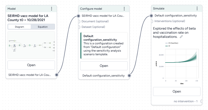
Simulate operator
In a workflow, the Simulate operator takes a model configuration and an optional intervention as inputs. Based on a customizable number of samples (to account for uncertainty) it outputs a set of simulation data.
-
Inputs
- Model configuration
- Intervention policies (optional)
-
Outputs
Simulation data
Add a Simulate operator to a workflow
-
Do one of the following actions:
- On an operator that outputs a model configuration or intervention policy, click Link > Simulate.
- Right-click anywhere on the workflow graph, select Simulation > Simulate, and then connect a model configuration to the Simulate input.
Simulate a model
The Simulate run settings allow you to fine-tune the time frame and solver behavior. By adjusting these settings, you can balance performance and precision.
Open a Simulate operator
- Make sure you've connected a model configuration to the Simulate operator.
- Click Open.
Configure the run settings
- Select a Preset, Fast or Normal.
-
Choose the End time to specify the simulation time range.
Note
If you included a starting timestep in your model configuration, the start and end dates also appear in your simulation.
Advanced settings
Using the following advanced settings, you can further optimize the computational efficiency and thoroughness of the simulation:
- Number of samples: Number of stochastic samples to generate.
-
Number of timepoints: Number of data points to generate over the simulation. Use this setting when you want to generate more timepoints than the duration of the simulation.
For example, a simulation with a duration of 10 days has 10 timepoints by default. Use this setting to increase or decrease the number of timepoints generated during the simulation.
-
Method: How to solve ordinary differential equations, dopri5 , rk4, or euler .
Tip
Using a low number of samples and the dopri5 method can speed up your runtime for debugging purposes.
Run the simulation
Once you've configured all the simulation settings, you can run the operator to generate a new simulation results dataset. The new dataset becomes a temporary output for the Simulate operator; you can connect it to other operators in the same workflow. If you want to use it in other workflows, you can save it for reuse.
Create a new simulation run
- Click Run.
Choose a different output for the Simulate operator
- Use the Select an output dropdown.
Save simulation results as a new dataset
- On the Simulate pane, click Save as new dataset.
View simulation results
When the simulation is complete, Terarium shows the results on the operator in the workflow and in the operator details. Available details include:
- An AI-generated description.
- Configurable charts.
- Data table of results.
AI-generated summaries of results
AI-generated summaries of simulation results describe:
- The simulation settings you selected.
- Trends in model parameters and states over time.
- The effects of any interventions on outcomes.
Edit the auto-generated summary
You can edit the summary to provide your own interpretation of the data.
- Click anywhere on the description, make your changes, and press Enter.
Charts
Configurable charts provide a visual way to understand and validate simulation results, allowing you to view interventions over time, compare variables and model states, and perform sensitivity analysis to see how parameter changes affect outcomes.
-
Interventions over time
These charts are only available if you connected an intervention policy to the Simulate input. For more information, see Simulate an intervention policy.
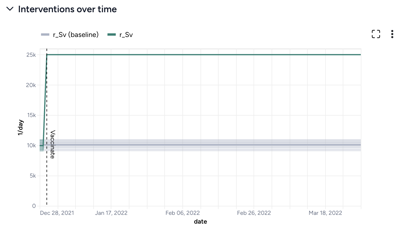
At day 2, vaccination rate increases from 10,000 people per day to 25,000 people per day. -
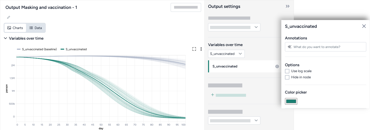
Variables over time
To aid visual validation, the variables over time charts compare the effects of simulation for state variables and observables.
-
Comparison charts
The comparison charts let you plot two or more parameters, model states, or observables to visualize how they differ over the course of the simulation.
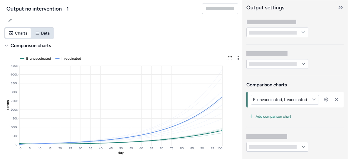
To access the following options for comparison charts, click Options in the Output settings.
Comparison method
Split the selected variables into separate Small multiples charts. You can further customize the small multiples charts to show the Same Y axis for all charts or Show before and after plots of the variables.
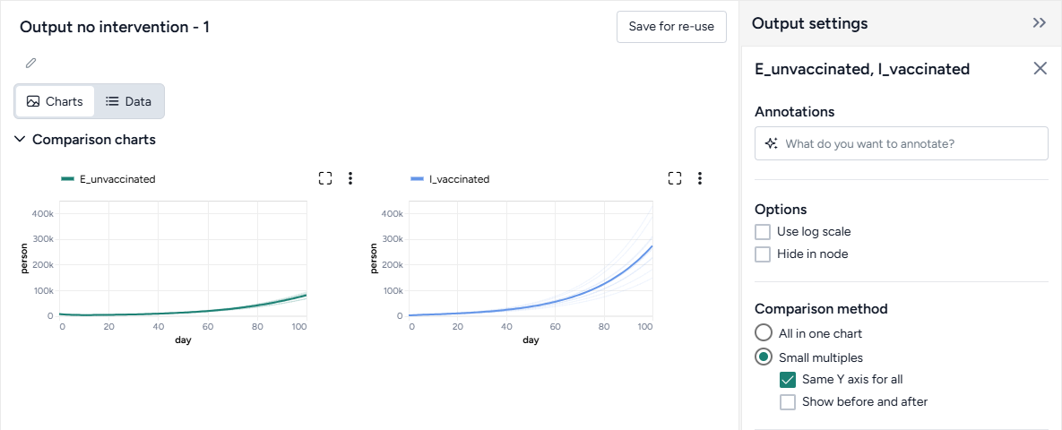
Use multiple charts if the variables you want to compare have very different ranges or values.
Normalization
Normalize data by total strata population to accurately assess the impact on each group regardless of size. With this option selected, the y-axis shows percentages, enabling comparisons across demographic segments by accounting for population size differences.
The equations used to normalize the charts appear below the setting.
-
Sensitivity analysis
Sensitivity analysis charts show how changes in model parameters affect the outcome variables of interest. For more information, see Sensitivity analysis.
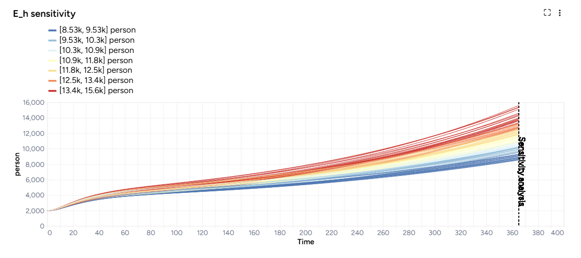
Sensitivity analysis graph showing the number of humans exposed to Mpox at day 365
Access the Output settings
Settings for the various chart types are available in the Output settings panel.
- Click Expand to expand the Output settings.
Choose which variables to plot
- Select the variables from the dropdown list.
Access additional chart settings
Some chart sections let you select additional options for each chart or variable. To access these settings:
- Click Options .
Annotate charts
Adding annotations to charts helps highlight key insights and guide interpretation of data. You can create annotations manually or using AI assistance.
Display options
You can customize the appearance of your charts to enhance readability and organization of the results.
Change the chart scale
By default, charts are shown in linear scale. You can switch to log scale to view large ranges, exponential trends, and improve visibility of small variations.
- Select or clear Use log scale.
Hide in node
The variables you choose to plot appear in the results panel and as thumbnails on the Simulate operator in the workflow. You can hide the thumbnail preview to minimize the space the Simulate node takes up.
- Select Hide in node.
Change parameter colors
You can change the color of any variable on the interventions over time, variables over time, and sensitivity charts to make your charts easier to read.
- Click the color picker and choose a new color from the palette or use the eye dropper to select a color shown on your screen.
Save charts
You can save Simulate charts for use outside of Terarium. Download charts as images that you can share or include in reports, or access structured JSON that you can edit with Vega .
Save a chart for use outside Terarium
- Click and then choose one of the following options:
- Save as SVG
- Save as PNG
- View source (Vega-Lite JSON)
- View compiled Vega (JSON)
- Open in Vega Editor
Data
An interactive table of simulation results enables you to explore model state and parameter values across various samples and timepoints, providing a detailed view of how these values evolve throughout the simulation.
View simulation data
- Click Data.
Troubleshooting
Recommended run settings
It's recommended you run simulations on the Normal Preset using the dopri5 Solver method.
Uncertainty and number of samples
If your models have no uncertainty in parameter values, only one sample is needed. Change Number of samples to 1 (the default is set to 100).
Simulation length and number of samples
If you plan to run your simulation for a long time or with a large number of samples (for example, End time or Number of samples > 100), set them to a lower value (10 or 20) first and run a check for errors.
Error messages
PyCIEMSS error messages should offer guidance on how to proceed. Error messages from Pyro or torchdiffeq may be less clear.
Cholesky factorization
If you see a message referencing Cholesky factorization (including The factorization could not be completed because the input is not positive-definite):
- There is an issue with the model, likely a model state blowing up to infinity or rapidly decreasing to negative infinity. Go back and check your model equations and configuration. Make sure the flow between compartments is correct, and then try adjusting your parameter values or initial conditions (are they too big?).
AssertionError
If the simulation fails and shows an AssertionError: underflow in dt 0.0 error, the configuration has made the model unsolvable with the selected solver Method. This often happens with the dopri5 solver method.
- Workaround: Try using a different solver method, such as rk4 or euler. These solvers are be less efficient than dopri5, but they are also less likely to get caught in an unworkable state