Terarium help
| Author(s) | Uncharted Software Inc. |
| Copyright | Copyright © 2025 Uncharted Software Inc. |
Home ↵
About Terarium
Terarium is a modeling and simulation workbench designed to help you assess and contribute to the scientific landscape. New to the workbench? Check out these topics:
Regardless of your level of programming experience, Terarium allows you to:
- Extract models from academic literature
- Parameterize and calibrate them
- Simulate a variety of scenarios
- Analyze the results
Need more help? Check out these topics:
Ended: Home
Get started ↵
Using Terarium
Terarium supports your scientific decision making by helping you organize, refine, and communicate the results of your modeling processes. You can:
- Gather existing knowledge.
- Break down complex scientific operations into separate, easy-to-configure tasks.
- Create reproducible visual representations of how your resources, processes, and results chain together.
How Terarium represents your modeling work
The following concepts describe how Terarium organizes your modeling work to help you manage, visualize, and run scientific processes.
-
Project
A workspace for storing modeling resources, organizing workflows, and recording and sharing results.
-
Resource
Scientific knowledge—models, datasets, or documents (PDF)—used to build workflows and extract insights.
-
Workflow
A visual canvas for building and capturing your modeling processes. Workflows show how resources move between different operators to produce results.
-
Operator
A part of a workflow that performs tasks like data transformation or simulation.
Creating a project
Create a project for a problem you want to model and then:
- Upload existing models, datasets, and documents to build a library of relevant knowledge.
- Visually construct different modeling workflows to transform the resources and test different models.
Create a project
- On the Home page, do one of the following actions:
- To start from scratch, click New project.
- To find a project to copy, search My projects or Public projects and then click > Copy.
- To upload a project, click Upload project and drag in or browse to the location of your .project file.
- In the new project, edit the overview to capture your goals and save results over time.
Gathering resources
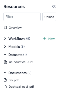
Use the Resources panel to upload and access your models, datasets, and documents.
Note
You can also add resources by:
- Copying them from other projects.
- Creating them using Terarium's library of operators.
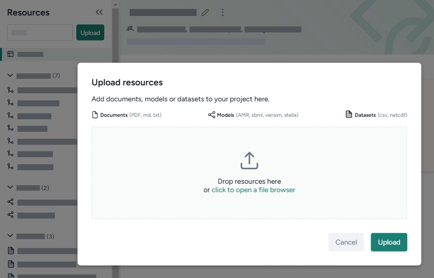
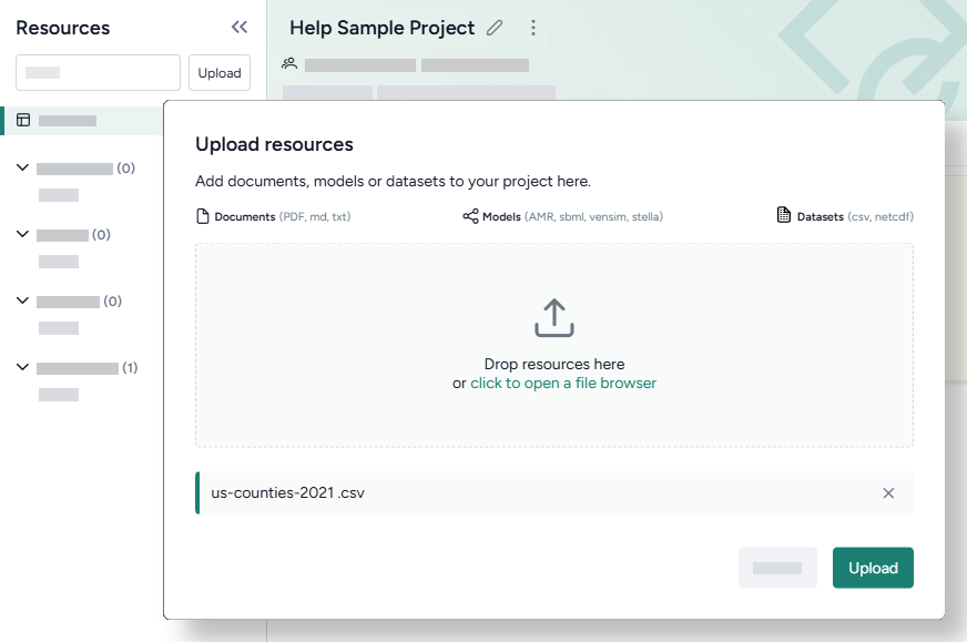
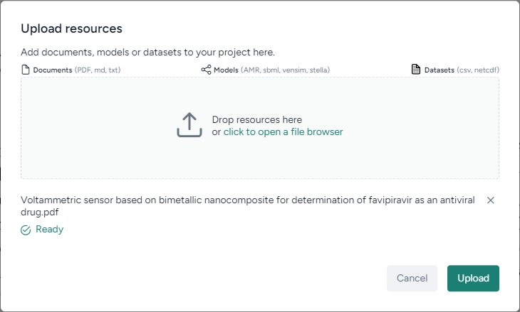
Upload resources
- Do one of the following actions:
- Drag your files into the Resources panel.
- Click Upload and then click open a file browser to navigate to the location of the files you want to add.
-
Click Upload.
Note
To view a resource, click its title in the Resources panel.
Building scientific modeling workflows
Create a workflow to visually build your modeling processes. Each box is a resource or an operator that handles a task like transformation and simulation. Chain their outputs and inputs to:
- Recreate, reuse, and modify existing models and datasets to suit your modeling needs.
- Rapidly create scenarios and interventions by configuring, validating, calibrating, and optimizing models.
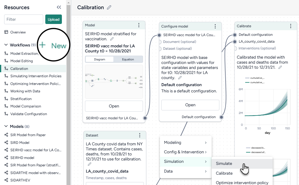
Create a workflow
- In the Workflows section of the Resource panel, click New.
- Select a template, fill out the required fields, and then click Create.
-
Use the canvas to customize your workflow:
- Drag in models, datasets, or documents from the Resources panel.
- Right-click on the canvas to add operators.
- Connect resources and operators by clicking the source input and followed by the output destination. Labels show you the types of resources and operators you can connect.


Using the library of operators
Terarium's operators support various ways for you to configure complex scientific tasks. For example, you can drill down to access:
- A guided wizard for quickly configuring common settings.
- A notebook for direct coding.
- An integrated AI assistant for creating and refining code even if you don't have any programming experience.
Use a Terarium operator
- Make sure you've connected all the required inputs.
- Click Open on the operator node.
-
Switch to the Wizard or Notebook view depending on your preference.
Note
Any changes you make in the Wizard view are automatically translated into code in the Notebook view.
-
Modeling
-
Create model from equations
Build a model using LaTeX expressions or equations extracted from a paper.
Source code -
Edit model
Modify model states and transitions using an AI assistant.
Source code overview -
Stratify model
Divide populations into subsets along characteristics such as age or location.
Source code overview -
Compare models
Generate side-by-side summaries of two or more models or prompt an AI assistant to visually compare them.
Source code overview
-
-
Simulation
- Simulate
Run a simulation of a model under specific conditions.
[Source code]https://github.com/ciemss/pyciemss/blob/e3d7d2216494bc0217517173520f99f3ba2a03ea/pyciemss/interfaces.py#L357){ target="_blank" rel="noopener noreferrer" } - Calibrate
Determine or update the value of model parameters given a reference dataset of observations.
Source code - Optimize intervention policy
Determine the optimal values for variables that minimize or maximize an intervention given some constraints.
Source code - Simulate ensemble
Run a simulation of multiple models or model configurations under specific conditions.
Source code - Calibrate ensemble
Extend the calibration process by working across multiple models simultaneously.
Source code
- Simulate
-
Data
-
Transform dataset
Modify a dataset by explaining your changes to an AI assistant.
Source code user guide -
Compare dataset
Compare the impacts of two or more interventions or rank interventions.
-
-
Config and intervention
- Configure model
Edit variables and parameters or extract them from a reference resource. - Validate configuration
Determine if a configuration generates valid outputs given a set of constraints.
Source code repository - Create intervention policy
Define intervention policies to specify changes in state variables or parameters at specific points in time.
- Configure model
Recreate, modify, and simulate a model
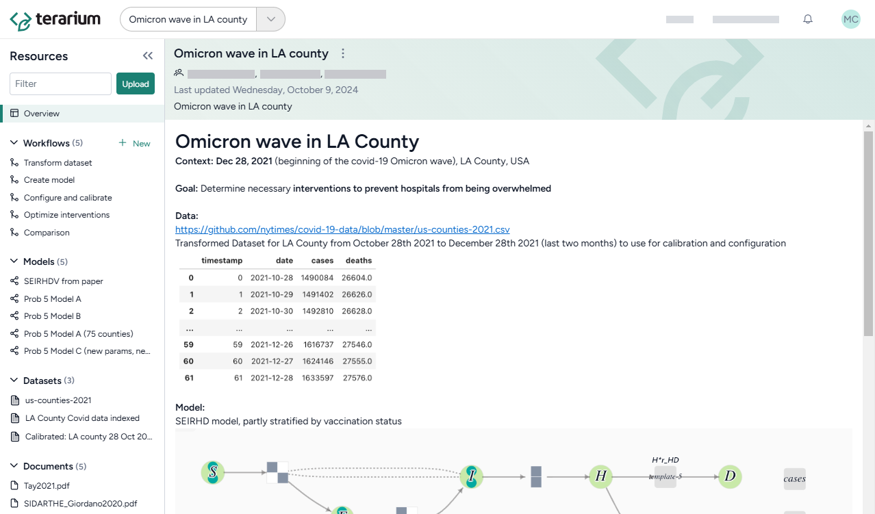
This tutorial is designed to help you learn how—all without needing to code—you can recreate, refine, and analyze models in Terarium. You can follow along by looking at the shared Terarium help sample project.
The goal of the modeling exercise in the project is to reduce COVID hospitalizations in LA county. Starting with only a dataset of cases and deaths and a few scientific papers describing disease models, it shows how to:
-
Upload and modify models and data
- Upload resources
- Create and compare models from equations
- Edit a model
- Stratify a model to account for dimensions like vaccination status
- Work with data
-
Simulate models and explore intervention policies
Try it out yourself!
To better understand the described modeling processes, see the sample workflow link at the top of each section. To try something out yourself, copy the models, documents, or datasets from the sample workflow into your own project.
To copy a model or dataset:
- Click its name in the Resources panel.
- Click > Add to project and select your project.
To copy a document:
- Click its name in the Resources panel.
- Click > Download this file and save it to your computer.
- Drag the file into the Resources panel of your prroject.
Upload and modify models and data
Upload resources
Begin setting up your project by uploading the models, papers (documents), and datasets you need for your modeling processes. In this case, that includes a dataset of U.S. COVID cases and deaths from 2021 and a set of papers describing different disease models.
Upload modeling resources
- Drag the dataset and document files into the Resources panel and then click Upload.
Create and compare models from equations
Terarium can automatically recreate a modelfrom a set of ordinary differential equations. In this case, we create models by extracting equations from the uploaded documents, but you could also get equations from pasted images or manually enter them as LaTeX.
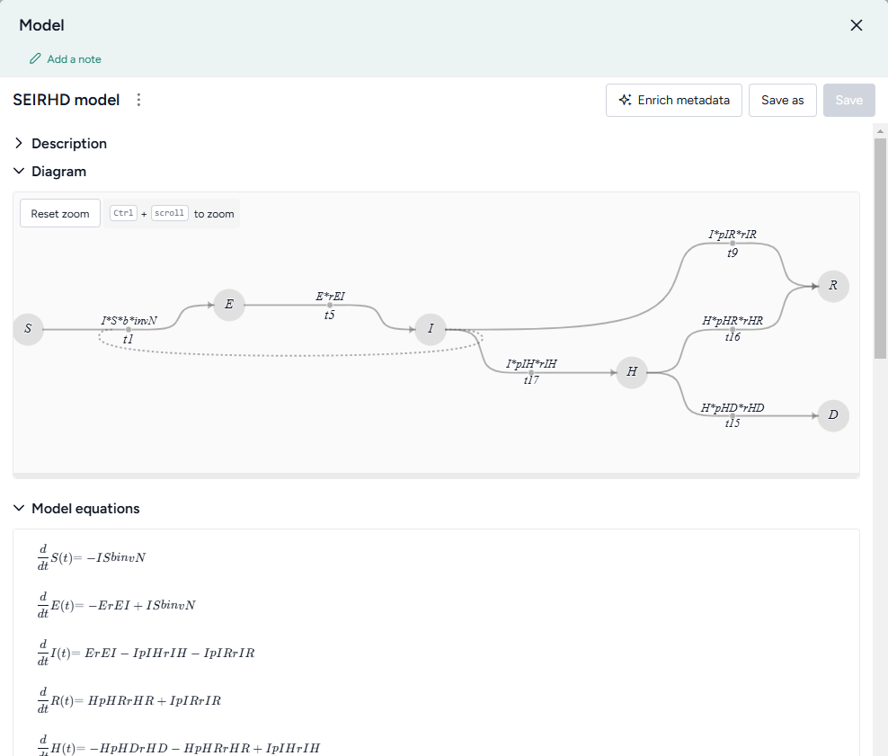
When the extraction and creation is complete, Terarium builds visual representations of the extracted SIR and SEIRHD models that show how people progress between disease states.
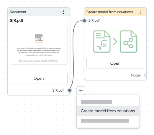
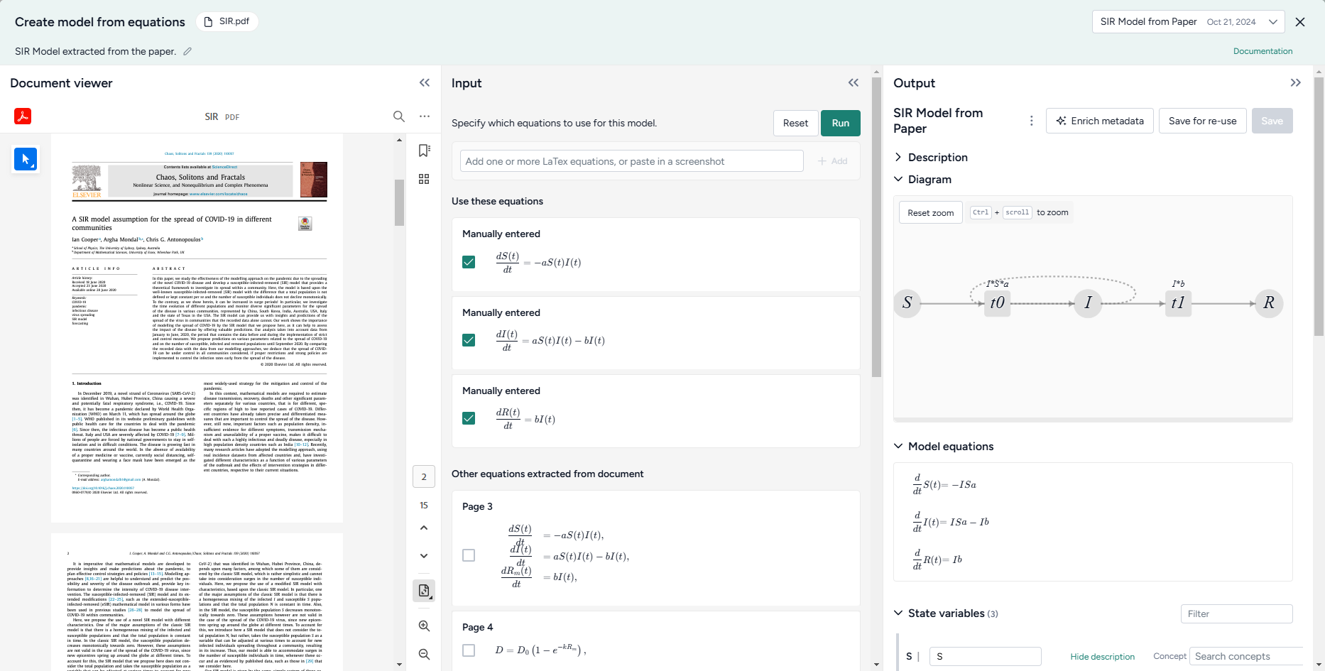
Recreate a model from a paper
- Drag each document into the workflow canvas, hover over its output, click Link > Create model from equations, and then click Open.
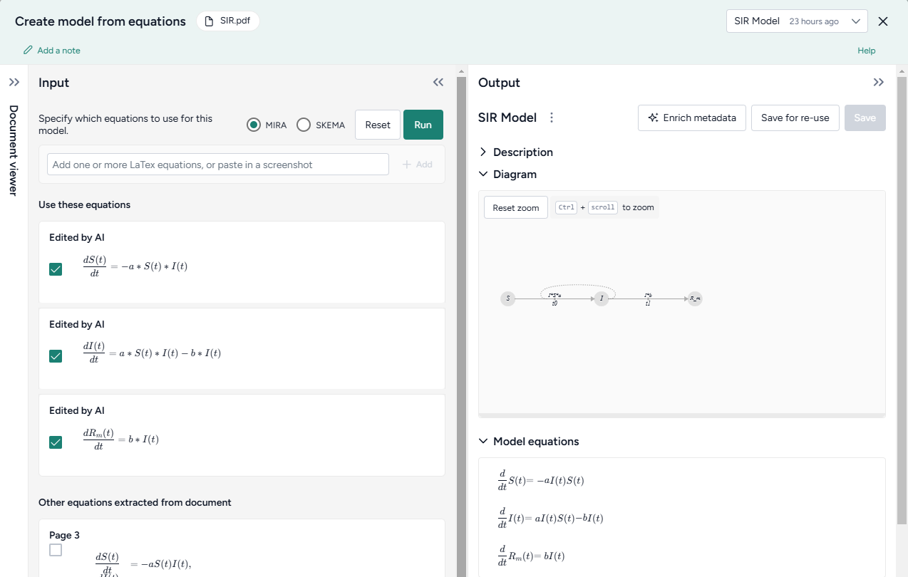
- Review the equations automatically extracted from the document. To make changes or correct extraction errors, click an equation to edit the LaTeX version.
- Select each equation you want to include in the model and then click Run > Mira.
- At the top of the Output panel, click Save for re-use, and then enter a unique name.
To understand the extracted SIR and SEIRHD models better and decide which one to use, we pipe them into a Compare models operator. This uses an AI assistant to create side-by-side model cards for each according to our modeling goal of reducing hospitalizations
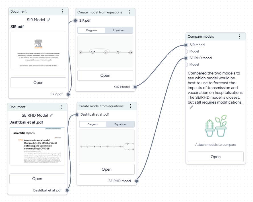
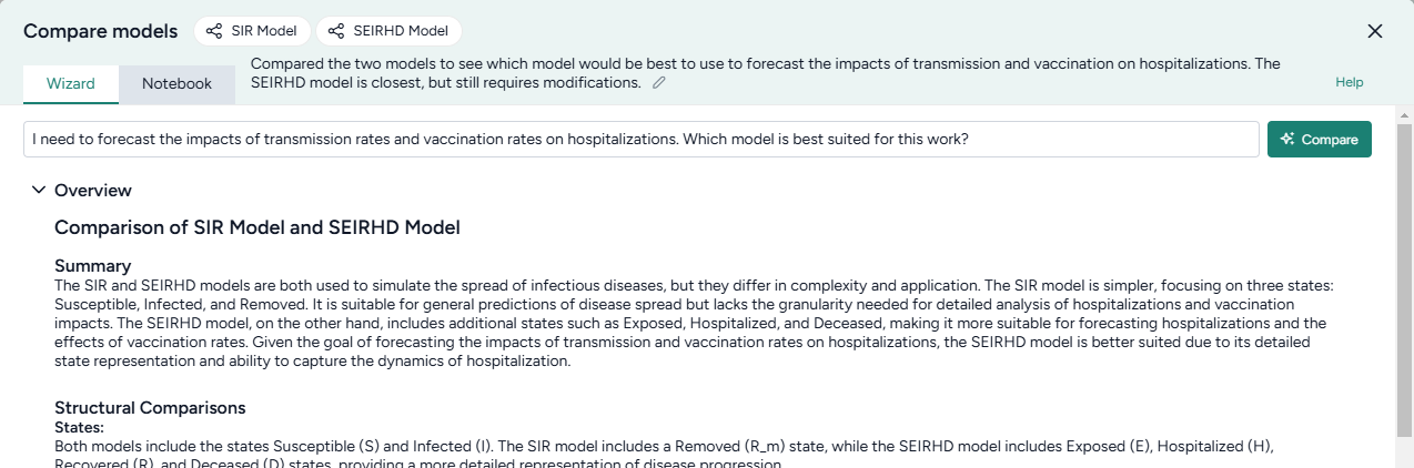
Compare models
- Hover the output of a Create model from equations operator and click Link > Compare models.
- Click the output of the other Create model from equations operator and connect it to the new Compare models operator.
- Click Open.
-
Enter your goal for making the comparison. In this case:
I need to forecast the impacts of transmission rates and vaccination rates on hospitalizations. Which model is best suited for this work?
-
Click Compare and review the summary tailored to the specified goal.
The AI-generated summary indicates that the SEIRHD model would be best for forecasting the impacts of transmission and vaccination on hospitalizations.
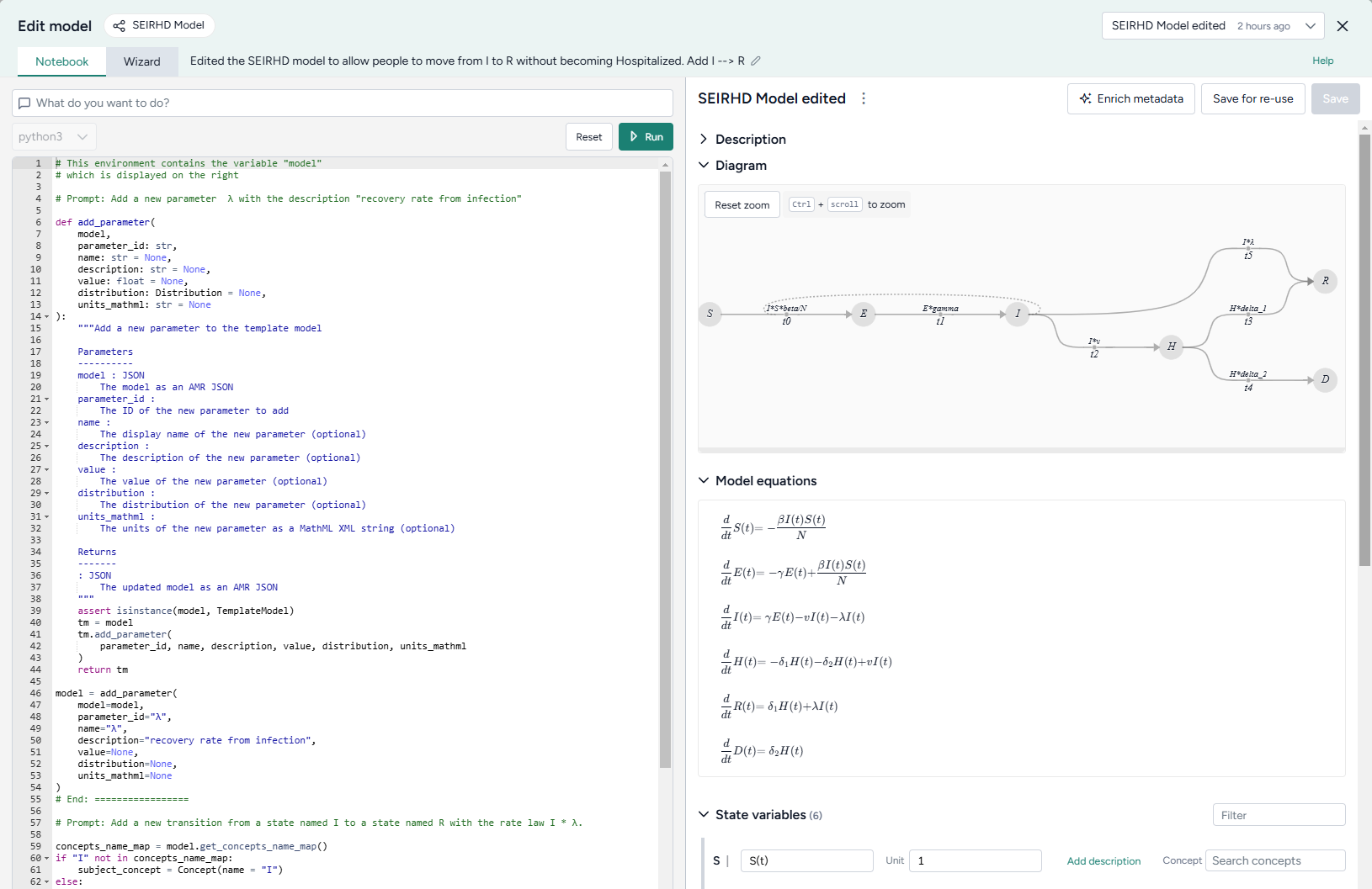
Edit models
Now we want to update the SEIRHD model to allow people to move from infected to recovered without becoming hospitalized. Even if you don't have any coding experience, you can use Terarium's AI-assisted Edit model notebook. The assistant simplifies the process of changing or building off an existing model—no knowledge of specialized modeling libraries needed!
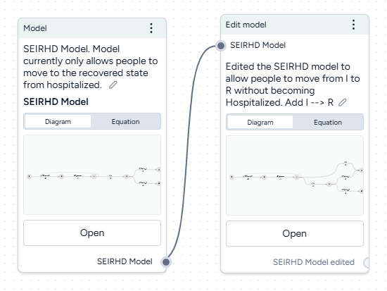
Add a new transition from infected to recovered
- Pipe the model into an Edit model operator and then click Open.
-
Add a new parameter for the transition rate law by asking the AI assistant to:
Add a new parameter λ with the description "recovery rate from infection" -
Add the new transition by asking the assistant to:
Add a new transition from a state named I to a state named R with the rate law I * λ -
Click Run to apply the changes. Compare the edited model to the previous state by changing the output in the top right.
- Click Save for re-use and then enter SEIRHD edited as the name of the new model.
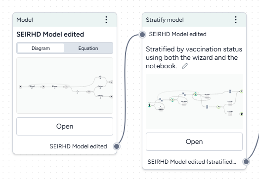
Stratify models
Now we want to stratify our edited model to account for vaccinated and unvaccinated groups. Terarium's stratification process is an error-proof approach to stratifying along any dimension, such as age, sex, and location.
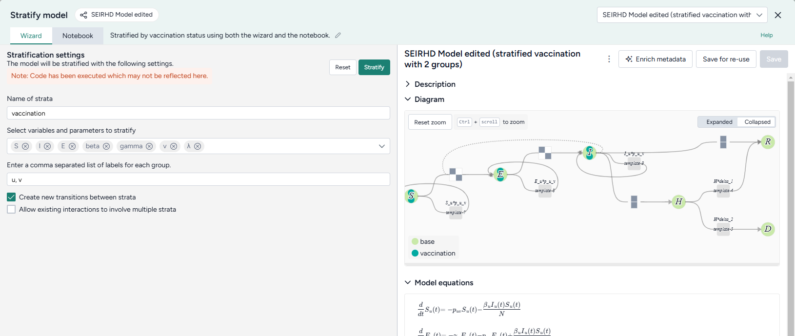
Stratify the SEIRHD model by age
- Pipe the model into an Stratify model operator and then click Open.
- Name the strata "vaccination".
- Select to stratify the S, E, and I state variables and the beta (infection rate), gamma (latent time), v (hospitalized rate), and λ (recovery rate) parameters.
-
List the labels for each strata group:
u, v -
Choose the allowed transitions and interactions between strata:
- Select Create new transitions between strata to allow unvaccinated people to turn into vaccinated people.
- Clear Allow existing interactions between strata to prevent vaccinated and unvaccinated people from interacting with and infecting each other.
Note
In this case because vaccinated people cannot turn into unvaccinated people, additional settings must be configured in the Notebook view. For more information, see the code inside the Stratify model operator in the Terarium help sample project or see Stratify a model.
-
Click Stratify.
- Click Save for re-use and edit the name of the new model.
Work with data
The uploaded dataset covers all of the U.S. for 2021. However, we're only interested in LA county. We can use Terarium's data transformation tools to filter down to just what we need.
We'll also add a timestep column, which we'll need later to calibrate our model to the historical data.
Filter the case data to focus on LA county
- Drag the dataset from the Resources panel onto the canvas, hover over its output, click link > Transform dataset, and then click Open.
- Preview the data by clicking Run .
-
Ask the assistant to filter the data:
filter the data for LA county from October 28th 2021 to December 28th 2021. Add a new column named timestep with the first value starting at 0 and increasing by n+1. -
Ask the assistant to plot the data over time:
plot cases over time for the filtered_df -
Inspect the generated code, change the following line to include
COVIDin the title, and then click Run to redraw the plot.plt.title('Number of Cases Over Time') -
Show the plot in the workflow by selecting Display on node thumbnail.
- At the top of the window, select filter_d1, click Save for reuse, and enter LA county cases and deaths as the name of the new dataset.
Doing your data transformations in Terarium helps make your modeling process more transparent and reproducible.
Simulate models and explore intervention policies
Configure and calibrate a model
Before you can simulate the modified SEIRHD model, we need to configure it to set the initial values for its states and parameters. To improve its performance, we can also adjust these by calibrating it against the context of the LA county data.
In this example, we'll work with an already existing model configuration, but normally you can manually create configurations based on your expert knowledge or automatically extract them from documents or datasets in your project.
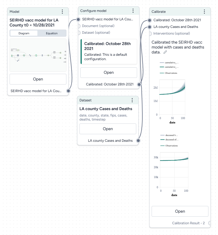
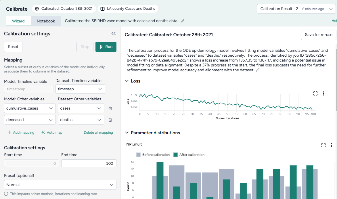
Calibrate the SEIRHD model to the LA county data
- Pipe the Configure model operator and the transformed dataset into a Calibrate operator and then click Open.
-
Map the model variables to the dataset variables:
- Set the Dataset: Timeline variable to timestep.
- Map model observables
cumulative casesanddeceasedto dataset variablescasesanddeathsrespectively.
-
Change the End time to 150 and click Run.
When you calibrate a model, you can review the following immediate visual feedback to help you spot issues quickly:
- A loss chart showing error over time.
- Cases and deaths data over time, with observations from the dataset and the projected number of cases before and after the calibration.
Run a sensitivity analysis
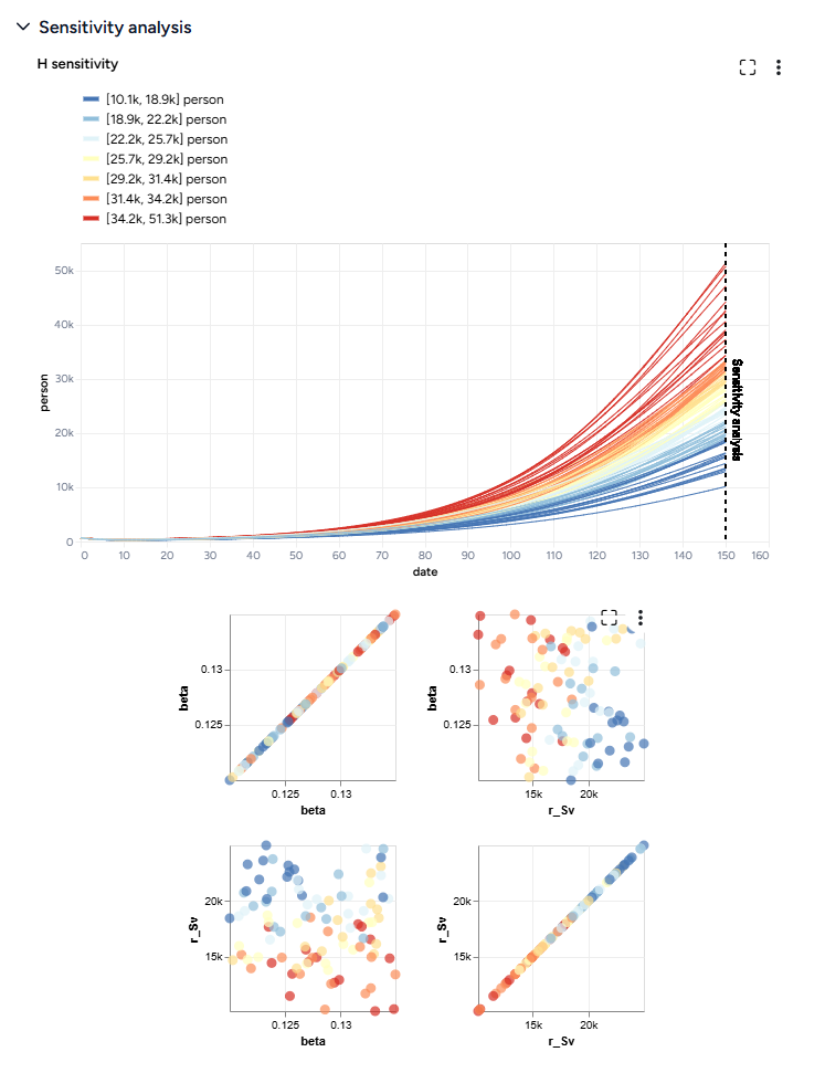
Next, we'll simulate our model configuration to perform a sensitivity analysis to explore the effects of infection rate (beta) and vaccination rate (r_Sv) on hospitalizations.
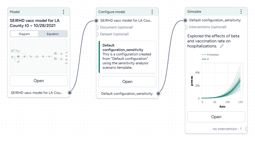
Run a sensitivity analysis with the Simulate operator
- Pipe the Configure model operator a Simulate operator and then click Open.
- Change the End time to 150 days and click Run.
The scatterplots below the sensitivity chart the parameters combine to affect hospitalizations shown in the chart above. Generally, high vaccination rates and low infection rates tend to reduce hospitalizations.
Create and simulate intervention policies
Our sensitivity analysis showed us the infection rates we should aim for to reduce hospitalizations. Now we can create different masking intervention policies to visualize the impact of different what-if masking scenarios that might get us there. For this, we'll use parameter NPI_mult, which is a multiplier for the transmission rate.
We'll create two policies:
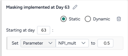
- One that sets NPI_mult to 50% on day 63.
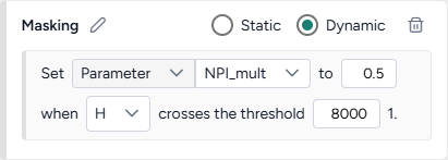
- One that sets to 50% only when hospitalizations cross 8,000.
Create and simulate an intervention policy to increase masking
- Pipe the Configure model operator into two different Create intervention policy operators and then click Open.
- Set the intervention policies:
- On one policy, create a new Static intervention starting at day 63 that sets Paramater NPI_mult to 0.5.
- On the other, create a new Dynamic intervention that sets Paramater NPI_mult to 0.5 when hospitalizations (H) cross the threshold of 8,000.
- Save each intervention policy and give them unique names.
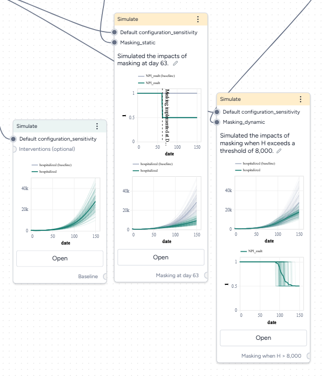
- Create three new Simulate operators:
- One the first, pipe in only the model configuration to get a baseline without interventions.
- On the second, pipe in the model configuration and the static intervention.
- On the third, pipe in the model configuration and the dynamic intervention.
- Open each Simulate operator, change the End time to 150 days, and click Run.
- Click Save for re-use to save each simulation result as a new dataset.
Both interventions reduce hospitalizations compared to the baseline, but the static intervention of introducing masking at day 63 is more effective than the dynamic intervention that waits for hospitalizations to reach 8,000.
Optimize intervention policies
In Terarium, you can optimize interventions to meet specified constraints, allowing you to get answers to key decision maker questions faster. We want to find how effective masking needs to be to prevent hospitalizations from exceeding capacity.
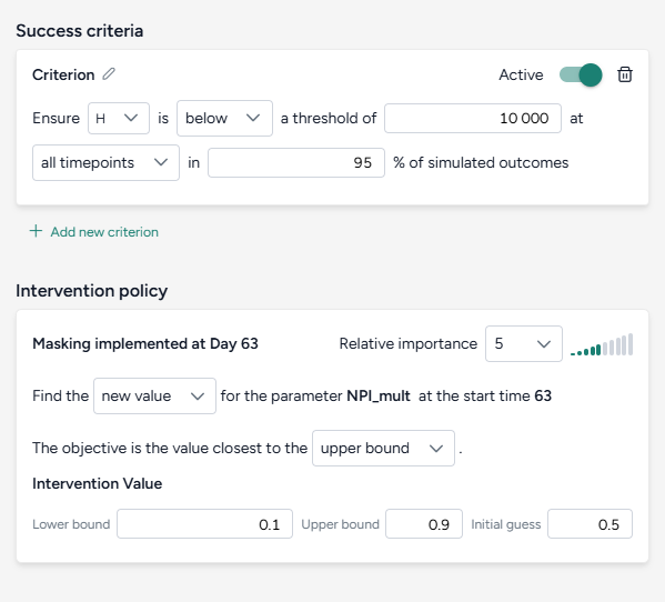
Optimize the intervention policy to find how effective masking needs to be to reduce hospitalizations
- Pipe the static intervention and model configuration into an Optimize intervention policy operator and click Open.
-
Set the success criteria:
- Ensure hospitalizations (H) are below 10,000 at all timepoints in 95% of simulated outcomes.
-
Specify a new intervention:
- Find a new value for the parameter NPI_mult with the objective being closest to the upper bound of the range from 10–90%.
- Set the initial guess to 50%.
-
Simulate for 150 days and click Run.
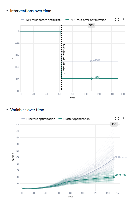
By simulating the optimized intervention policy, you can see how the estimates of masking compliance affect peak hospitalizations:
- Initial guess: NPI_mult of 50%, which leads to peak hospitalizations of 9,602.
- Optimization: NPI_mult of 20.7%, which leads to peak hospitalizations of 4,071.
Compare datasets
Finally, you can take the results of your simulations, interventions, and optimizations and compare them to see which works best at reducing hospitalizations. The Compare datasets operator lets you compare scenarios based on the various simulation results you've generated.
Optimize the intervention policy to find how effective masking needs to be to reduce hospitalizations
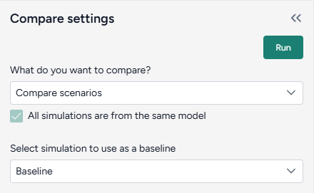
- Pipe the datasets you created from simulating your different intervention policies into a Compare datasets operator and click Open.
- Select Compare scenarios, choose the baseline dataset, and click Run.
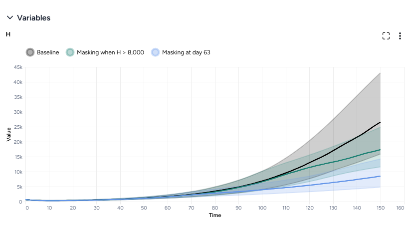
- In the Output settings, select H (hospitalizations) to plot the variable over time for each of the datasets.
You can see the effectiveness of the different intervention policies on a single plot. Starting masking at day 63 is most effective at reducing hospitalizations.
What's next?
We've completed the sample SEIRHD model workflow! You now have the tools you need to start uploading, transforming, and simulating models and model resources in Terarium.
Instructional videos
The following videos show how to use Terarium to, for example:
- Create models.
- Edit models.
- Work with data.
- Run what-if scenarios.
- Calibrate models.
- Create, simulate, and optimize intervention policies.
- Stratify models.
Introduction
Working with data
Creating a model from equations
Editing a model
Calibration
Simulating intervention policies
Optimizing intervention policies
Stratification
Ended: Get started
Gather modeling resources
With Terarium, you can gather, store and manage resources needed for your modeling and simulation workflows. You can pull in documents, models, and datasets from:
Documents, models, and datasets appear in your project resources. You can transform and simulate them by dragging them into a workflow.
Upload resources
Using the Resources panel, you can import resources of the following types:
-
Documents
- PDF files (.PDF)
- Markdown files (.MD)
- Text files (.TXT)
Note
Uploaded documents run through an extraction process that, depending on the size of the PDF, may take some time.
-
Models
- PetriNet models in Systems Biology Markup Language (SBML) format (.XML or .SBML)
- Terarium model and model configuration formats (.JSON and .modelconfig)
- StockFlow models in Vensim format (.MDL)
- StockFlow models in Stella formats (.XMILE, .ITMX, .STMX)
-
Datasets
- Comma-separated values (.CSV)
- NetCDF (.NC)
Upload resources
- Do one of the following actions:
- Drag your files into the Resources panel.
- Click Upload and then click open a file browser to navigate to the location of the files you want to add.
- Click Upload.
PDF Extraction
Most resources you upload are available for use right away. When you upload a PDF document however, Terarium begins extracting any linear ordinary differential equations it finds in the text. Depending on the size of the PDF, this process can take some time.
Note
The extractor isn't optimized to handle every way that equations can represent models. Before using any extracted equations to create a model from equations, check and edit them if necessary.
Check the status of a PDF extraction
- Click Notifications .
Search for and copy resources from other projects
You can get resources by copying them from other projects in Terarium. If you know their location, you can get them directly from the source project. Otherwise, use the project search on the home page to find relevant resources.
Find projects containing resources of interest
The project search finds projects and resources by keyword. Keywords are checked against the names of projects and resources such as models, datasets, documents, model configurations, intervention policies, and workflows.
- Click the Terarium logo to return to the home page.
- Enter your keywords in the search field and press Enter.
- In the results, click the project name to view the source project overview or click the resource name to open it.
Get a model or dataset from another project
- Open the project that contains the model or dataset.
- Open the model or dataset by clicking its name in the Resources panel.
- Next to the model or dataset name, click > Add to project and select your project.
Get a document from another project
- Open the project that contains the document.
- Open the document by clicking its name in the Resources panel.
- Click > Download this file and save it to your computer.
- Open your project and reupload the document.
Build a workflow graph
A workflow is a visual canvas for building and running complex operations (calibration, simulation, and stratification) on models and data.
Create a new blank workflow
- In the Resources panel, click New in the Workflows section.
- Enter a name for the workflow and click Create.
Create a new workflow based on a template
- In the Resources panel, click New in the Workflows section.
- Select the template for the type of workflow you want to create.
-
Enter a name for the workflow, set the required inputs and outputs, and then click Create.
Note
Before you can use a template, your project must contain the inputs (models, model configurations, or datasets) you want to use.
Create new workflows based on templates
The following workflow templates streamline the process of building common modeling workflows. They provide preconfigured and linked resources and operators tailored to your objectives, such as analyzing uncertainty, forecasting potential outcomes, or comparing intervention strategies.
Note
- Before you can fill out a template, your project must contain the inputs (models, model configurations, or datasets) you want to use.
- Before you can see the results of a templated workflow, you must configure and run any Calibrate, Simulate, or Compare datasets operators it contains.
- You can create new intervention policies with the template. Once the workflow is created, you must create the Create intervention policy operator and add your intervention criteria.
Situational awareness
Use this template to determine what's likely to happen next. For example, you can:
- Anticipate the arrival of a new variants.
- Evaluate the potential impact of growing vaccine hesitancy and declining Non-Pharmaceutical Interventions (NPIs).
Fill out the Situational awareness template
To use the Situational awareness template, select the following inputs and outputs:
-
Inputs
- Model
- Model configuration
- Dataset
-
Outputs
- Metrics (model states) of interest
Complete the Situational awareness workflow
The new workflow first calibrates the model to historical data to obtain the best estimate of parameters for the present. Then it forecasts the model into the near future. To see the results, you first need to open the Calibrate operator and:
- Map the model variables to the dataset columns.
- Run the calibration.
This creates:
- Charts comparing the selected model states before and after calibration with observations from the dataset.
- A new model calibrated to the dataset.
Sensitivity analysis
Use this template to determine which model parameters introduce the most uncertainty in your outcomes of interest. For example, you can explore:
- Unknown severity of new variant.
- Unknown speed of waning immunity.
Fill out the Sensitivity analysis template
To use the Situational awareness template, select the following inputs and outputs:
-
Inputs
- Model
- Model configuration
- One or more uncertain parameters of interest and the ranges to explore
- Simulation settings (optional)
-
Outputs
- Metrics (model states) of interest
Complete the Sensitivity analysis workflow
The new workflow first configures the model with parameter distributions that reflect all the sources of uncertainty. Then it simulates the model into into near future. To see the results, you first need to open the Simulate operator, edit any settings, and run it. This creates:
- A sensitivity analysis chart for each selected model state and pairwise comparison charts for each selected parameter.
- A simulation results dataset.
Decision making
Use this template to determine the impact of different interventions. For example, you can find:
- The impact of several combinations of vaccination and Non-Pharmaceutical Interventions (NPIs) levels.
- Whether it's better to implement an intervention in all locations, select locations, or not at all.
Fill out the Decision making template
To use the Decision making template, select the following inputs and outputs:
-
Inputs
- Model
- Model configuration
- One or more intervention policies
- Simulation settings (optional)
-
Outputs
- Metrics (model states) of interest
Complete the Decision making workflow
The new workflow first runs simulations for the baseline (no intervention) and each intervention policy. It then compares the relative impact of each intervention policy to the baseline. To see the results, you first need to:
- Open and run each Simulate operator.
- Open and run the Compare datasets operator.
This creates a comparison of the simulated baseline and intervention policies.
Horizon scanning
Use this template to determine how extreme scenarios impact the outcome of different interventions. For example, you can explore:
- Potential emergence of a new variant.
- Rapidly waning immunity.
Fill out the Horizon scanning template
To use the Horizon scanning template, select the following inputs and outputs:
-
Inputs
- Model
- Model configuration
- One or more uncertain parameters of interest and the ranges to explore
- One or more intervention policies (optional)
- Simulation settings (optional)
-
Outputs
- Metrics (model states) of interest
Complete the Horizon scanning workflow
The new workflow first configures the model to represent the cartesian product of the extremes of uncertainty for some parameters. It then simulates into the near future with different intervention policies and compares the outcomes. To see the results, you first need to:
- Open and run each Simulate operator.
- Open and run the Compare datasets operator.
This creates a comparison of the simulated extreme scenarios.
Value of information
Use this template to determine how uncertainty impacts the outcomes of different interventions. For example, you can determine whether:
- Uncertainty in severity changes the priority of which group to target for vaccination.
- Disease severity impacts the outcome of different social distancing policies.
Fill out the Value of information template
To use the Value of information template, select the following inputs and outputs:
-
Inputs
- Model
- Model configuration
- One or more uncertain parameters of interest and the ranges to explore
- One or more intervention policies
- Simulation settings (optional)
-
Outputs
- Metrics (model states) of interest
Complete the Value of information workflow
The new workflow first configures the model with parameter distributions that reflect all the sources of uncertainty. It then simulates into the near future with different intervention policies. To see the results, you first need to:
- Open and run each Simulate operator.
- Open and run the Compare datasets operator.
This creates a comparison of the uncertainty across the different interventions.
Reproduce models from literature
Use this template to reproduce models from literature and then compare them to find the best starting point. For example, you can determine whether:
- The results from a paper are reproducible.
- The best model from a group of recent papers to explore disease transmission.
Fill out the Reproduce models from literature template
To use the Reproduce models from literature template, select the following inputs and outputs:
-
Inputs
- One or more documents
- A brief description of your goal for comparing the resulting models (optional)
-
Outputs
- New models extracted from the documents
- Model configurations for each model
- Comparison of the models tailored to your goal
- Simulation results for the selected model configurations
Complete the Reproduce models from literature workflow
The new workflow first extracts the models from the documents. It then compares the models according to your goal and configures and simulates them into the near future. To see the results, you first need to:
- Open each Create model from equations operator, select the relevant equations from the paper, and run the operator to create the model.
- Open and run the Compare datasets operator.
- Open and edit the Configure model operators.
- Open and run the Simulate operators.
Calibrate an ensemble model
Use this template to create a more accurate model by combining multiple models in an ensemble. For example, you can determine how to:
- Leverage the strengths of each model to make the most accurate model possible.
Fill out the Calibrate an ensemble model template
To use the Calibrate an ensemble model template, select the following inputs and outputs:
-
Inputs
- A historical dataset
- Two or more models, each with their own model configurations
- A mapping of the timestamp values that the dataset and models share
- Additional mappings for each variable of interest that the dataset and models share
-
Outputs
- Simulation results each selected model configuration
- Calibrations against the historical for each of the selected model configurations
- Calibrated ensemble model based on each of the calibrations
Complete the Calibrate an ensemble model workflow
The new workflow first simulates and calibrates each model individually, then calibrates the ensemble. To see the results, you first need to:
- Open and run each Simulate operator.
- Open and run each Calibrate operator.
- Open and run the Calibrate ensemble operator.
Add resources and operators to a workflow
Workflows consist of resources (models, datasets, and documents) that you can feed into a series of operators that transform or simulate them.
Each resource or operator is a "node" with a title, thumbnail preview, and a set of inputs and outputs.
Add a resource to the workflow
- Drag the model, dataset, or document in from the Resources panel.
Add an operator to the workflow
Perform one of the following actions:
- Right-click anywhere on the graph and then select an operation from the menu.
- Click Add component and then select the operation from the list.
Connect resources and operators
Inputs and outputs on nodes let you resources and operators together to form complex model operations.
Connect resources and operators already in the workflow
- Click the output of one resource or operator and then click the corresponding input on another operator.
Example
- To configure a Calibrate operation to use a dataset, first click the output on the right side of the Dataset operator and then click the Dataset input on the left side of the Calibrate operator.
Connect resources and operators to a new operator
- Hover over the output of the resource or operator, click Link , and then select an operator.
Remove a connection between resources and operators
- Hover over the input or output and click Unlink.
Operators with yellow headers
An operator with a yellow header indicates that a resource or indicator that flows into it has changed and the operator needs to be rerun.
Edit resource and operator details
Resources and operators in the workflow graph summarize the data and inputs/outputs that they represent. You can drill down to view more details or settings.
View resource or operator details
Perform one of the following actions:
- Click Open.
- Click > Open in new window.
Duplicate a resource or operator
- Click > Duplicate
Manage a workflow
To organize your workflow graph, you can move, rearrange, or remove any of the operators.
Save a workflow
Terarium automatically saves the state of your workflow as you make changes.
Rename a workflow
- Click > Rename, type a unique name for the workflow, and press Enter.
Move a workflow operator
- Click the title of the operator and drag it to another location on the graph.
Remove a workflow operator
- Click > Remove.
Zoom to fit workflow
You can quickly zoom the canvas to fit your whole workflow to the current window.
Note
In some cases, parts of your workflow may be just off screen after the zoom.
- Click Reset zoom.
Review and transform data ↵
Working with data
You can use uploaded datasets or simulation results to configure and calibrate models. If the data doesn't align with your intended analysis, you can transform it by:
- Creating new variables
- Calculating summary statistics
- Filtering data
- Joining datasets
The Transform data operator can also serve as a place to visually plot and compare multiple datasets or simulation results.
Note
For information about uploading datasets, see Gather modeling resources.
Dataset resource
A dataset resource can represent:
- A dataset you've uploaded.
- A dataset you've modified and saved.
- The output of a simulation or an optimized intervention policy.
In a workflow graph, a dataset resource lists the columns it contains. You can use it to:
- Open and explore the raw data.
- Run data transformations, model configurations, and model calibrations.
-
Inputs
- None
-
Outputs
- Dataset
Add a dataset resource to a workflow
- Drag the resource from the Datasets section of the Resources panel.
What can I do with a dataset resource?
Hover over the output of the Dataset resource and click link to use the dataset as an input to one of the following operators.
-
Data
- Transform dataset
Guide an AI assistant to modify or visualize the dataset. - Compare dataset
Compare the impacts of two or more interventions or rank interventions.
- Transform dataset
-
Configuration and intervention
- Configure model
Use the dataset to extract initial values and parameters for the condition you want to test. - Validate configuration
Use the dataset to validate a configuration.
- Configure model
-
Simulation
- Calibrate
Use the dataset to improve the performance of a model by updating the value of configuration parameters. - Calibrate ensemble
Fit a model composed of several other models to the dataset.
- Calibrate
Review and enrich a dataset
Once you have uploaded a dataset into your project, you can open it to:
- Explore and summarize its data and columns.
- Manually add metadata that explains the data in each column.
- Automatically enrich metadata using documents in your dataset or without additional context.
Review a dataset
To get an understanding of your data, you can open a dataset and review its columns and a selection of its rows. A dataset resource previews up to 100 rows of data.
Open a dataset
-
Perform one of the following actions:
- In the Resources panel, click the name of the dataset.
- On a Dataset node in the workflow graph, click Open.
View the raw data in a dataset
- Click Data in the navigation list on the right.
Download a dataset
- Next to the dataset name, click > Download.
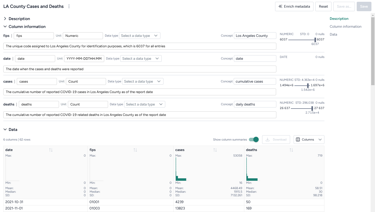
Enrich a dataset
If your dataset lacks descriptive details about what each column contains, you can use Terarium's dataset enrichment capability to complete the:
- Units: What the column measures (dates, cases, people) or contains (text).
- Descriptions: A short plain language explanation of the column's contents.
- Concepts: Epidemiological concepts that relate to the data in the column. Helpful in mapping data to model variables.
- Distributions of values
Terarium's enrichment service uses an AI language model to generate column details based on either:
- Contextual clues in the contents of a document in your project.
- The column headers in the dataset. In this case, the language model attempts to define the columns as if they relate to a general epidemiological context.
Note
- Curating concepts improves structural comparison and alignment of models and data.
- If Terarium can't determine what a column represents, it fills out the description to summarize distribution of values it contains.
Enrich dataset metadata
- Click Enrich metadata.
-
Perform one of the following actions:
- To enrich metadata without selecting a document, click Generate information without context.
- To use a document, select the document title.
-
Click Enrich.
- Review the updated description and column information.
- Click Save.
Add or edit dataset metadata
- Edit the Name, Unit, Data type, Concept, or Description of any field.
- Click Save.
Transform a dataset
If a dataset doesn't align with your modeling goals, you can transform it by cleaning and modifying it or combining it with other datasets. Supported transformations include:
-
Manipulation
- Creating new variables.
- Filtering the data.
- Joining two or more datasets.
- Performing mathematical operations.
- Adding or dropping columns.
- Sorting the data.
- Handling missing values.
- Converting incidence data (such as daily new case counts) to prevalence data (total case counts at any given time).
-
Visualization and summarization
- Calculating summary statistics.
- Describing the dataset.
- Plotting the data.
- Answering specific questions about the data.
The Transform dataset operator is a code notebook with an interactive AI assistant. You describe in plain language the changes you want to make, and the large language model (LLM)-powered assistant automatically generates the code for you.
Note
The Transform dataset operator adapts to your level of coding experience. You can:
- Work exclusively by prompting the assistant with plain language.
- Edit and rerun any of the assistant-generated code.
- Enter your own executable code to make custom transformations.
Transform dataset operator
In a workflow, the Transform dataset operator takes one or more datasets or simulation results as inputs and outputs a transformed dataset.
Tip
For complex transformations with multiple steps, it can be helpful to chain multiple Transform dataset operators together. This allows you to:
- Keep each notebook short and readable.
- Isolate transformations that take a long time so you don't have to rerun them multiple times.
- Access intermediate results for testing or comparison.
You can choose any step in your transformation process as the thumbnail preview.
Add the Transform dataset operator to a workflow
-
Perform one of the following actions:
- On a resource or operator that outputs a dataset, hover over the output and click Link > Transform dataset.
- Right-click anywhere on the workflow graph, select Data > Transform dataset, and then connect the output of one or more Datasets or Simulations to the Transform dataset inputs.
Modify data in the Transform dataset code notebook
Inside the Transform dataset operator is a code notebook. In the notebook, you can prompt an AI assistant to answer questions about or modify your data. If you're comfortable writing code, you can edit anything the assistant creates or add your own custom code.
Prompts and responses are written to cells where you can preview, edit, and run code. Each cell builds on the previous ones, letting you gradually make complex changes and save the history of your work. You can insert prompts or cells at any point in the chain of transformations.
Tip
Wait until the status of the AI assistant is Ready (not Offline or Busy) before attempting to make any transformations.
 Ready (not
  Offline or
  Busy) before attempting to make any transformations.
 Open the Transform dataset code notebook
- Make sure you've connected one or more datasets to the Transform dataset operator and then click Open.
Rerun a code notebook
When you reopen a Transform dataset notebook, the code environment is completely fresh. The initial datasets may be preloaded, but none of the transformations you previously made will be. To load them all:
- Click Rerun all cells.
Reset the kernel
From time to time, the AI assistant may get caught in a loop or stuck in a long-running transformation. To reset it:
Note
Resetting the kernel doesn't delete your prompts or the code cells in the notebook. You can still access and reload them at any time.
- Click Reset kernel.
- To reload the transformations in the notebook, click Rerun all cells.
Prompt the AI assistant to transform data
The Transform dataset AI assistant interprets plain language to answer questions about or transform your data.
Tip
The AI assistant can perform more than one command at a time.
Prompt or question the AI assistant
- Click in the text box at the top of the page and then perform one of the following actions:
- Select a suggested prompt and edit it to fit your dataset and the transformation you want to make.
- Enter a question or describe the transformation you want to make.
- Click Submit .
- Scroll down to the new code cell to inspect the transformation.
Choose where to insert a prompt
By default, new prompts and responses appear at the bottom of the notebook. To go back and insert intermediate steps in your transformation, you can change where your prompts appear. Note that if you do this, you will need to rerun any downstream transformations.
- Select the cell above where you want to insert the new prompt and response.
- Submit your new prompt.
How to write better prompts
The AI assistant generates better code when given specific instructions. Unintended actions or hallucinations are more likely to occur when instructions are vague. Describe what you want in steps, and clearly identify source datasets, columns, and actions.
The assistant often doesn't create previews or new datasets unless prompted. Include in your prompts whether you want to:
-
Preview your data:
Add a new column that keeps a running total of infections. Show me the first 10 rows. -
Create an intermediate dataset:
Create a new dataset named "result". The first column is named "fips" and its values are...
If you're not satisfied with a response, you can generate a new one or modify your prompt to refine what you'd like to see.
Tip
If the assistant doesn't produce the desired results, you can keep your transformation process well organized by adding more details to your prompt and then regenerating the responses. This ensures that any unnecessary results don't get saved in the notebook.
Change your prompt
- Click Edit prompt, change the text as needed, and then press Enter.
Get a new response to your prompt
- Click > Re-run answer.
How the AI assistant interprets prompts
To give you a sense whether it correctly interpreted your prompt, the assistant:
- Records its thoughts about your prompt (
I need to filter the dataset to only include rows with location equal to 'US'). - Shows how it intends to perform the transformation (
DatasetToolset.generate_python_code). - Presents commented code that explains what it's done.
When the response is complete, the code cell may also contain:
- A direct answer to your question.
- A preview of the transformed data.
- Any applicable error codes.
- Any requested visualizations.
Show or hide the assistant's thoughts about your prompt
- Click Show/Hide thoughts.
Add or edit code
At any time, you can edit the code generated by the AI assistant or enter your own custom code. The notebook environment supports the following languages, each extended with commonly used data manipulation and scientific operation libraries.
Note
The use of Julia is currently disabled.
-
Python libraries
- pandas for organizing, cleaning, and analyzing data tables and time series.
- numpy for handling of large arrays of numbers and performing mathematical operations.
- scipy for performing advanced scientific operations, including optimization, integration, and interpolation.
- pickle for saving and reloading complex data structures.
-
Julia libraries
- DataFrames for manipulating data tables.
- CSV for reading, writing, and processing CSV files.
- HTTP for sending and receiving data over the Internet.
- JSON3 for working with JSON data.
- DisplayAs for displaying data.
-
R libraries
- data.frame for manipulating data tables.
Tip
More libraries are available in the code notebook, but you may need to import them before use.
-
To list the available packages, click Add a cell and then enter and run:
pip listPkg.installed()installed.packages() -
To import a package, click Add a cell and then enter and run:
import <package_name>using <package_name>library(<package_name>)
Additional libraries that may be useful for data transformations
-
Data manipulation and analysis
-
Data visualization
- cartopy for creating maps and visualizing geographic data.
- matplotlib for creating static, animated, and interactive visualizations.
-
Machine learning
- scikit-learn for creating machine learning models.
- torch for building, training, and experimenting with machine learning models.
-
Image processing
- scikit-image for processing and analyzing images.
-
Graph and network analysis
- networkx for working with networks and graphs.
Change the language of the code notebook
The Transform dataset AI assistant writes Python code by default. You can switch between Python, R, or Julia code at any time.
- Use the language dropdown above the code cells.
Make changes to a transformation
- Directly edit the code in the In cell and then click Run .
Add your own custom code
- Scroll to the bottom of the window and click Add a cell.
- Enter your code in the In cell and then click Run .
Choose where to insert your custom code
By default, new code cells appear at the bottom of the notebook. You can add intermediate steps in your transformation by changing where your code cells appear. Note that if you do this, you will need to rerun any downstream transformations.
- Select the cell above where you want to insert the new code cell.
- Click Add a cell.
Save transformed data
At times in your transformation or whenever specifically prompted, the AI assistant creates new transformed datasets as the output for the Transform dataset operator. This lets you return to previous versions of your dataset or choose the best one to save and use in your workflow.
When you're done making changes, you can connect the chosen output to any operators in the same workflow that take datasets as an input.
To use a transformed dataset in other workflows, save it as a project resource.
Choose a different output for the Transform dataset operator
- Use the Select a dataframe dropdown.
Save a transformed dataset to your project resources
You can save your transformations as a new dataset at any time.
- (Optional) If you created multiple outputs during your transformations, Select a dataframe to save.
- Click Save for reuse, enter a unique name in the text box, and then click Save.
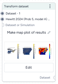
Preview a transformation on the Transform dataset operator in the workflow graph
- Select Display on node thumbnail.
Download a transformed dataset
- Save the transformation output as a new dataset.
- Close the Transform dataset code notebook.
- In the Resources panel, click the name of the new dataset.
- Click > Download.
Transformation examples
The following sections show examples of how to prompt the Transform dataset AI assistant to perform commonly used transformations.
Example prompts
Some simple prompts that can be used as part of larger transformation processes include:
Filter the data to just location = "US"Convert the date column to timestamps and plot the dataCreate a new census column that is a rolling sum of 'value' over the previous 10 daysAdd a new column that is the cumulative sum of the valuesPlot the dataRename column 'cases' to 'I', column 'hospitalizations' to 'H', and 'deaths' to 'E'
Clean a dataset
You can use the AI assistant to clean your dataset by specifying column types, reformatting dates, and performing other common data preparation tasks.
Specify the type of data in a column
Reformat a column of numeric IDs to, for example, add back leading zeroes that were stripped off:
Set the data type of the column "fips" to "string". Add leading zeros to the "fips" column to a length of 5 characters.
Reformat dates
Datasets with inconsistent date formats can interfere with accurate interpretation and integration into model parameters:
Set the data type of the column "t0" to datetime with format like YYYY-MM-DD hh:mm:ss UTC
Combine datasets
Before you combine datasets, make sure they share at least one common column like name, ID, date, or location. You can ask the AI assistant to link them by matching records based on the common data so that information aligns correctly.
- Connect the outputs of each dataset to the input of a Transform dataset operator and then click Open.
-
Ask the assistant to:
Join d1 and d2 where date, county, and state match. Save the result as a new dataset and show me the first 10 rows.Tip
You can also specify what type of join (such as inner join, left join, right join, or full outer join) you want the assistant to perform.
-
To save the dataset as a new resource in your project, change the dataframe and click Save for reuse.
Plot a dataset
You can visualize your data to explore patterns, compare quantities, identify relationships, analyze distributions, and capture insights tailored your analysis. Supported visualizations include:
- Line plots
- Bar charts
- Scatter plots
- Box plots
- Histograms
- Pie charts
- Heatmaps
- Violin plots
- Bubble charts
- Area charts
Tip
To refine your visualizations, edit your prompt to add more details about what you want to see (for example, add Insert a legend to a prompt that initially only requests a plot).
-
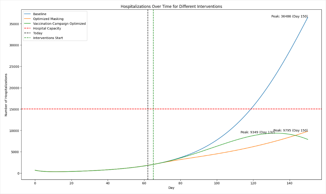
Ask the assistant to plot your data. For the best results, be as specific as possible about what you want to see:
plot the number of hospitalizations over the 150 days for the baseline, masking, and vaccination interventions. -
To refine the visualization, perform one of the following actions:
- Edit your prompt to add more information that explains the changes you want.
- Edit the generated code and then click Run .
-
(Optional) To share the image:
- Select Display on node thumbnail to use the image as the thumbnail on the Transform dataset operator in the workflow.
- Right-click the image, select Copy image, and then paste it into your project overview.
Create a map-based visualization
The AI assistant can connect to third-party code repositories and data visualization libraries to incorporate geolocation data and then create map plots.
These prompts ask the assistant to get U.S. county-level data from plotly and then use using matplotlib and geopandas handle and visualize geographic data structures.
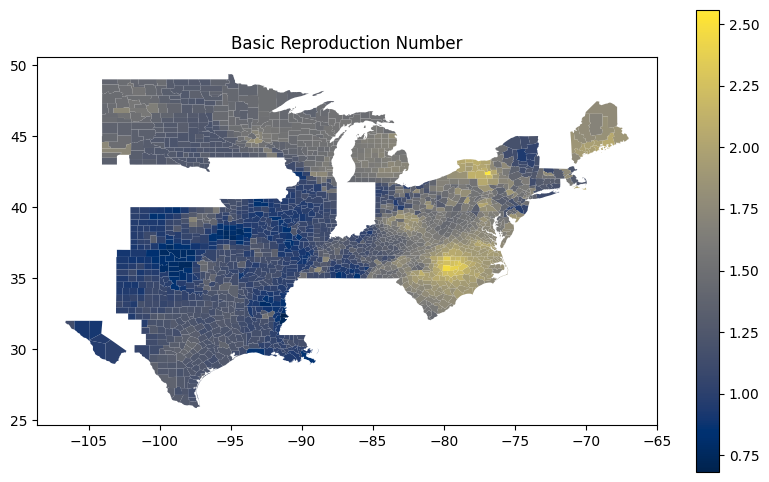
Write me code that downloads the US counties geojson from plotly GitHub using urlopen
Use matplotlib to make a figure. Create a choropleth map from the column "Rl" in the geopandas dataframe "new_df_all". Use the "cividis" colormap. Add a legend.
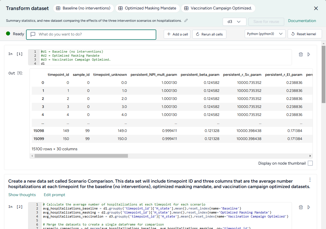
Compare datasets
You can use the AI assistant to compare multiple datasets or simulation results.
See the Working with Data workflow in the Terarium Sample Project. It takes three datasets generated by optimizing intervention policies and then:
- Combines them into a new scenario comparison dataset.
- Calculates summary statistics for hospitalizations in each dataset.
- Identifies the timepoint at which the maximum number of hospitalizations occur in each dataset.
- In a separate data transformation, plots hospitalizations for each intervention over time.
Convert incidence data to prevalence data
If you have an epidemiological dataset that contains incidence data (such as new cases per day), you can prompt the AI assistant to convert it to prevalence data (such as total cases at any given time). You will need to specify:
- How long it takes people to recover.
- The susceptible population.
This prompt converts daily case counts into prevalence data. It uses user-supplied recovery and population data to calculate total cases:
let's assume avg time to recover is 14 days and time to exit hosp is 10 days. Can you convert this data into **prevalence** data? please map it to SIRHD. Assume a population of 150 million.
For more information on the logic of how the AI assistant converts from incidence to prevalence data, see the instructions the assistant follows in these cases.
Calculate peak times
Calculating peak times can help you identify critical periods of disease spread, enabling targeted interventions.
This prompt takes a collection of daily infection rates for various FIPs codes and identifies the peak time for each one:
Create a column named "peak_time". The first column is "fips". The second column is "peak_time", and its values are the values of the "timepoint" column for which the values of the FIPS columns are at a maximum.
Compare datasets
You can compare the impacts of two or more interventions or rank interventions using the Compare datasets operator.
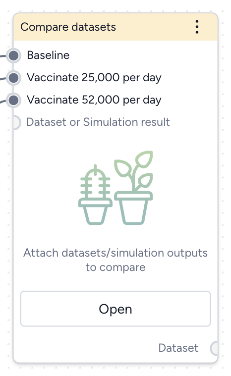
Compare datasets operator
In a workflow, the Compare datasets operator takes two or more datasets or simulation results as inputs and plots them. It outputs a dataset comparison, which can be used as a dataset in other operators.
-
Inputs
Two or more datasets or simulation results
Tip
Use descriptive names for your datasets and simulation results. This will help you interpret the comparison.
-
Outputs
Dataset comparison
Add the Compare datasets operator to a workflow
-
Perform one of the following actions:
- On a resource or operator that outputs a dataset or simulation result, click Link > Compare datasets.
- Right-click anywhere on the workflow graph, select Data > Compare datasets, and then connect the output of two or more datasets or simulation results to the Compare datasets inputs.
Compare datasets
You can visually compare the impact of interventions or rank interventions based on multiple criteria.
Open the Compare datasets operator
- Make sure you've connected two or more datasets or simulation results to the Compare datasets operator and then click Open.
Compare the impact of interventions
You can assess how different interventions influence outcomes by directly comparing their effects on key variables.
Define the comparison
You can set up your dataset comparison by selecting a baseline and adjusting key options to align with your analysis goals.
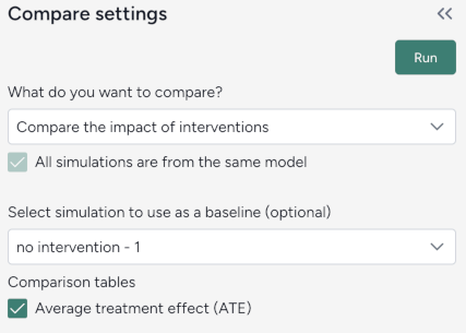
Define the comparison
- Select Compare scenarios.
- (Optional) Specify which dataset is the baseline simulation.
- (Optional) Select Average treatment effect to include a summary of the overall impact of interventions in the resulting comparison tables.
Customize the comparison plot
You can tailor the resulting comparison plots to highlight the most relevant aspects of your interventions.
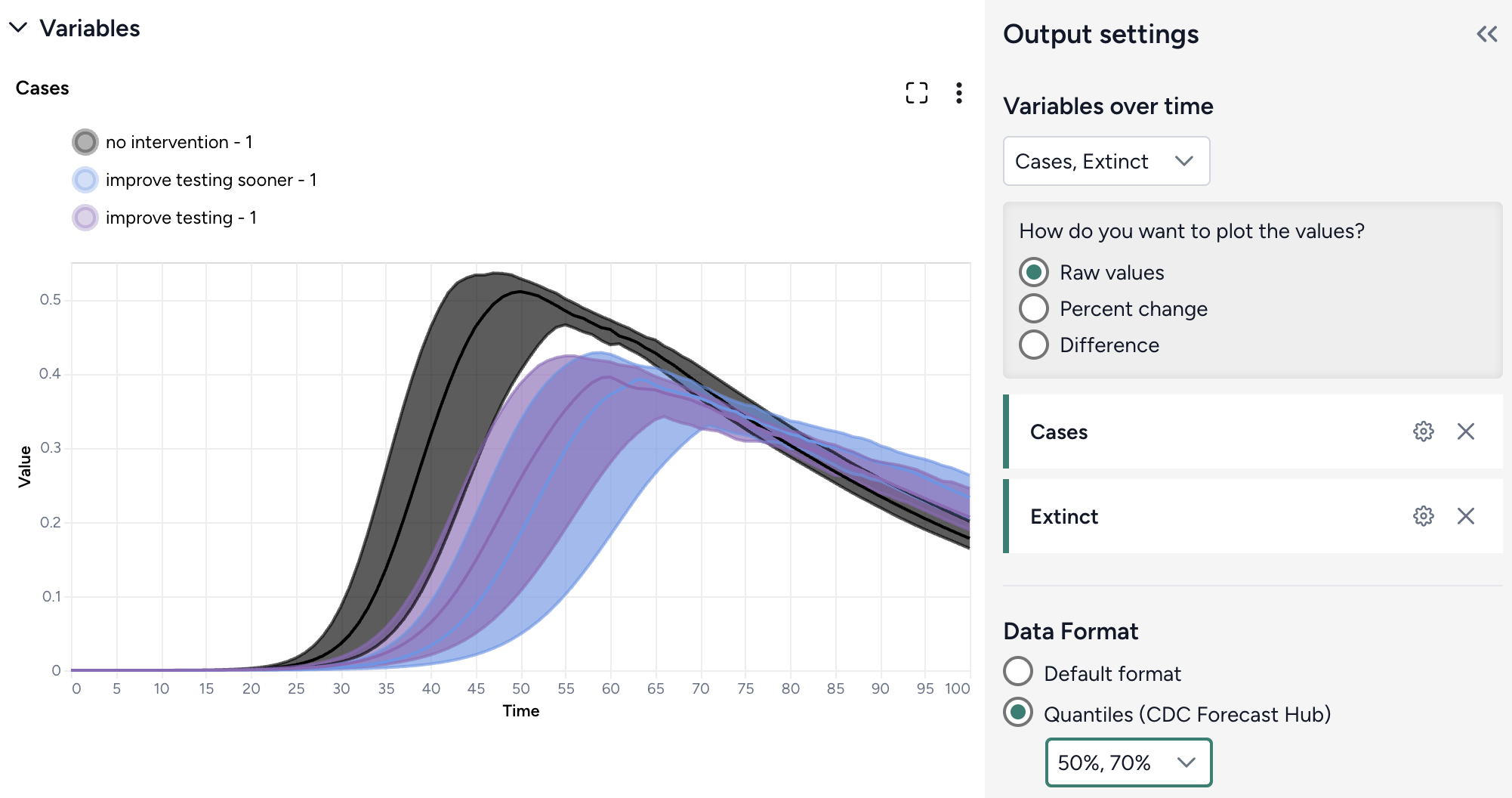
Customize the comparison plots
- Select the variables you want to plot.
-
Select how to plot the values. You can show:
- Raw values.
- Percent change with respect to the baseline.
- Difference from the baseline.
-
Select the data format to be displayed in the plot:
- Default (mean)
- Quantiles (specify upper and lower bounds).
Annotate charts
Adding annotations to charts helps highlight key insights and guide interpretation of data. You can create annotations manually or using AI assistance.
Add annotations that call out key values and timesteps
To highlight notable findings, you can manually add annotations that label plotted values at key timesteps.
- Click anywhere on the chart to add a callout.
- To add more callouts without clearing the first one, hold down Shift and click a new area of the chart.
Prompt an AI assistant to add chart annotations
You can prompt an AI assistant to automatically create annotations on the variables over time and comparison charts. Annotations are labelled or unlabelled lines that mark specific timestamps or peak values. Examples of AI-assisted annotations are listed below.
- Click Options .
-
Describe the annotations you want to add and press Enter.
Draw a vertical line at day 100Draw a line at the peak S after calibrationDraw a horizontal line at the peak of default configuration Susceptible after calibration. Label it as "important"```{ .text .wrap } Draw a line at x = 40 only for ensemble after calibrationDraw a vertical line at x is 10. Don't add the label
Display options
You can customize the appearance of your charts to enhance readability and organization of the results.
Access additional chart settings
To access additional options for each chart:
- Click Options .
Change the chart scale
By default, charts are shown in linear scale. You can switch to log scale to view large ranges, exponential trends, and improve visibility of small variations.
- Select or clear Use log scale.
Hide in node
The variables you choose to plot appear in the results panel and as thumbnails on the Compare datasets operator in the workflow. You can hide the thumbnail preview to minimize the space the Compare datasets node takes up.
- Select Hide in node.
Change parameter colors
You can change the color of any variable to make your charts easier to read.
- Click the color picker and choose a new color from the palette or use the eye dropper to select a color shown on your screen.
Rank interventions
More info coming soon.
Ended: Review and transform data
Modeling ↵
Working with a model
A model is an abstract representation that approximates the behavior of a system. In Terarium, you can build a chain of complex operations to recreate, edit, configure, stratify, calibrate, and simulate models.
Note
For information about:
- Uploading models, see Gather modeling resources.
- Creating models, see Edit model.
Model resource
A model resource represents a model you've uploaded to or created in Terarium.
In a workflow graph, a model resource shows its underlying diagram or equations. You can use the resource to:
- Open, review, and enrich the model variables, parameters, observables, and transitions.
- Edit or stratify the model.
- Compare it to other models.
- Create model configurations or intervention policies.
-
Inputs
- None
-
Outputs
- Model
Add a model resource to a workflow
- Drag the resource from the Models section of the Resources panel.
Copy a model
- Add the Model operator to a workflow graph and connect it to an Edit model operator.
- Click Open on the Edit model operator.
- Click Save for re-use, enter a name for the copy, and click Save.
What can I do with a model resource?
Hover over the output of the model resource and click link to use the model as an input to one of the following operators.
-
Modeling
- Edit model: Add, remove, or change state variables, transitions, parameters, rate laws, and observables.
- Stratify model: Divide populations into subsets along demographic characteristics such as age and location.
- Compare models: Compare side-by-side with other models to understand their similarities and differences.
-
Configuration and intervention
- Configure model: Set the initial values and parameters for the condition you want to test
- Create intervention policy: Create static and dynamic interventions for "what-if" scenarios.
Review and enrich a model
Once you have uploaded or created a model in your project, you can open it to:
- Explore its diagram, equations, state variables, parameters, observables, and transitions.
- Manually add metadata that explains the model components.
- Automatically enrich metadata using documents in your dataset or without additional context.
Review a model
To get an understanding of a model, you can open a detailed view that summarizes the following extracted details:
- Description
- Diagram
- Model equations
- State variables
- Parameters
- Observables
- Transitions
- Time
Open a model
- Click the model name in the Resources panel.
Download a model
- Next to the model name, click > Download.
Rename a model
- Click > Rename, type a unique name for the model, and press Enter.
Enrich model metadata
If your model lacks descriptive details about its variables and parameters, you can use Terarium's model enrichment capability to complete the:
- Names: A meaningful label that describes what the variable or parameter stands for.
-
Units: What the variable or parameter measures (people, cases).
Note
Transitions don't have units.
-
Descriptions: A short plain language explanation of the variable or parameter's contents.
- Concepts: Epidemiological concepts related to the variable or parameter. Useful for comparing models and mapping variables and parameters to data columns.
Note
Enrichment can also provide geolocation information if, for example, your model is stratified by geographic areas such as states or territories.
Terarium's enrichment service uses an AI language model to automatically populate model metadata based on either:
- Contextual clues in the contents of a document in your project.
- The variable or parameter names in the model. In this case, the language model attempts to define the metadata as if they relate to a general epidemiological context.
Enrich model metadata
- Click Enrich metadata.
-
Perform one of the following actions:
- To enrich metadata without selecting a document, click Generate information without context.
- To use a document, select the document title.
-
Click Enrich.
- Review the updated metadata.
- Click Save.
Add or edit model metadata
- Edit the Name, Unit, Description, or Concept.
- Click Save.
Create a model from equations
The Create model from equations operator helps you to recreate a model from literature or build a new model from LaTeX equations . In this process, you:
- Choose or enter the equations you want to include in the model.
- Create the model as an output or resource for use in other modeling and configuration processes.
Note
When you upload a document to your project, Terarium automatically extracts any ordinary differential equations it contains and converts them to LaTeX. However, the extraction doesn't handle all the ways that equations can represent models. Before using any equations, check and edit them if needed.
Create model from equations operator
In a workflow, the Create model from equations operator takes an optional document as an input and outputs a new model. You can use the operator without any inputs by entering or uploading LaTeX equations that represent the model you want to create.
Once you have created a model, the operator in the workflow shows its underlying diagram or equations.
How it works: Model Service
-
Inputs
Document (optional)
-
Outputs
Add the Create model from equations operator to a workflow
-
Perform one of the following actions:
- Hover over the output of a Document and click Link > Create model from equations.
-
Right-click the workflow graph and select Modeling > Create models from equations.
If needed, connect the output of a Document to the Create model from equations input.
Choose the equations
You can create a model from a set of ordinary differential equations by:
- Selecting equations from a document in your project.
- Uploading and extracting equations from an image.
- Manually entering equations as LaTeX code.
To ensure the best results, Terarium uses a set of LaTeX formatting guidelines when converting extracted equations. It is recommended that you follow these guidelines for any LaTeX you add or edit as well.
Select equations from a document
To recreate a model from literature, you can select any ordinary differential equations extracted from an input document. Terarium represents each equation as LaTeX.
In some cases you may want to change the LaTeX either to correct or and new details. As you edit the LaTeX, the equation is automatically updated.
Select equations from a document
- In the workflow, make sure the document is connected to the operator input and then click Open.
- In the Input panel, review and select the equations you want to include in the model.
Edit equations extracted from a document
Note
When you modify equations extracted from a document, your changes are only saved to the current Create model from equations operator. If you reuse the document in another Create model from equations operator, you need to make the edits again.
- Click an equation to jump to where it's found in the document and reveal the converted LaTeX code.
- Edit the code as necessary and verify that the updated equation matches your edits.
- Select the check box next to the equation to include it in the model.
Extract equations from an image
In some cases, Terarium may not extract all the equations you want from a document. Or you may have equations from other sources that you want to bring into your project. In these cases, you can capture a screenshot of the equations and load them into Terarium for automatic extraction.
Extract equations from an image
- Take a screenshot of the equations you want to use or copy a saved image of the equations.
- Click inside the text box and paste your image. For example, right click and select Paste or press Ctrl+V.
- Click Add.
- Review the new equations. Click to reveal the LaTeX code and edit it if necessary.
Enter your own equations
In addition to selecting extracted equations, you can also paste or enter LaTeX code from elsewhere.
Manually enter equations
- Use the text box to add LaTeX equations to enter a new equation and click Add.
- Repeat step 1 for each equation you want to add.
Manually copy an equation from a document
If the automatic extraction missed an equation from your document, you can still copy it and add it separately.
- Select the text in the document viewer and then click Copy text.
- Paste the equation into the Input text box and edit as necessary.
- Click Add.
Recommended LaTeX format
The Create model from equations operator works with LaTeX equations. Before it creates a model, Terarium uses an AI assistant to "clean" your edited equations according to the following guidelines. You can follow these same guidelines yourself or enter equations as you normally would and then check the AI-cleaned equations for errors such as missing terms or duplicated parameters.
-
Derivatives
-
Write derivatives in Leibniz notation, not Newton or Lagrange notation.
Recommended:
\frac{d X}{d t}
Not recommended:\dot{X}
Not recommended:X^\primeorX' -
Represent partial derivatives of one-variable functions as ordinary derivatives.
Recommended:
\frac{d X}{d t}
Not recommended:\partial_t X
Not recommended:\frac{\partial X}{\partial t} -
Place first-order derivatives to the left of the equal sign.
-
-
Mathematical notations
- Avoid the use of:
- Capital sigma (
Σ) and pi (Π) notations for summation and product. - Non-ASCII characters.
- Homoglyphs (characters that look similar but have different meanings).
- Capital sigma (
-
To indicate multiplication, use
*.Recommended:
"b * S(t) * I(t)Not recommended:b S(t) I(t) -
Rewrite expressions with negative exponents as explicit fractions.
Recommended:
"\frac1{{ N }}Not recommended:N^1
- Avoid the use of:
-
Parentheses
- When grouping algebraic expressions, don't use square brackets
[ ], curly braces{ }, or angle brackets< >. Use parentheses( )if needed. -
Always expand expressions surrounded by parentheses using the order of mathematical operations.
Recommended:
\alpha * x(t) * y(t) + \beta * x(t) * z(t)Not recommended:x(t) (\alpha y(t) + \beta z(t))
- When grouping algebraic expressions, don't use square brackets
-
Variable and symbol usage
-
For variables that have time
tdependence, write the dependence explicitly as(t),Recommended:
X(t)
Not recommended:X -
For variables and names, avoid the use of words or multiple character.
- If needed, use camel case (
susceptiblePopulationSize) to combine multi-word or multi-character names. - Replace any variant form of Greek letters (
\varepsilon) with their main form (\epsilon) when representing a parameter or variable. - Don't separate equations by punctuation (commas, periods, or semicolons).
-
-
Superscripts and subscripts
- To denote indices, use LaTeX subscripts
_instead of superscripts and LaTeX superscripts^. - Use LaTeX subscripts
_instead of Unicode subscripts. Wrap all characters in the subscript in curly brackets{...}.
- To denote indices, use LaTeX subscripts
Create the model
Once you have selected the equations you want to use, you can create a new model as:
- An output you can connect to other operators in the same workflow.
- A project resource that you can use in any of your workflows.
- A downloadable JSON file you can use in external tools.
Note
Before it creates a model, Terarium uses an AI assistant to "clean" the selected equations according to the LaTeX formatting guidelines. When the model is ready, the Input panel shows the equations "Edited by AI" that appear in the model.
Create a new model from the selected equations
When you run the Create model from equations operator, the newly created model becomes an output you can connect to other operations in the same workflow.
-
Click Run.
Run options for creating models
Terarium supports two methods for creating models from equations:
- MIRA uses LLM assistance to standardize LaTeX equations , translate them to SymPy equations , and then create a Petri Net model.
- SKEMA uses regular expressions to rigidly parse LaTeX equations and create a Petri Net model.
MIRA is the default and recommended model. SKEMA can be used as a workaround when MIRA generates errors or inaccurate results. SKEMA is most reliable for equations with no parentheses, no production/degradation, and no complex rate law expressions.
-
Review the new equations. If you need to make changes, edit the equations in the Input panel and click Run again.
- If needed, use the Output panel to enrich the model metadata and then click Save.
Save the new model as a resource for use in other workflows
By default, the new model only appears as an output of the Create new model. You can make it available for use in other workflows by saving it as a project resource.
- In the Output panel, click Save for re-use and choose a name for the new model.
Download the new model
- Next to the model name, click > Download.
Edit a model
Model editing lets you build on existing models. Supported edits include:
- Answering questions about, adding, removing, or changing state variables, transitions, parameters, rate laws, and observables.
- Renaming model elements.
- Setting variable or parameter units.
- Replacing parameters with more complex formulas.
- Resetting the model to its original state.
The Edit model operator is a code notebook with an interactive AI assistant. You describe in plain language the changes you want to make, and the large language model (LLM)-powered assistant automatically generates the code for you.
Note
The Edit model operator adapts to your coding experience. You can:
- Use plain language to prompt an AI assistant for a no-code experience.
- Edit and rerun AI-generated code.
- Write own executable code to make custom edits.
Note
For more examples and information about model editing, see the MIRA training material.
Edit model operator
In a workflow, the Edit model operator takes a model or model configuration as an input and outputs an edited model.
Tip
For complex edits with multiple steps, it can be helpful to chain multiple Edit model operators together. This allows you to:
- Keep each notebook short and readable.
- Access intermediate results for testing or comparison.
Once you've completed your edits, the thumbnail preview shows the diagram or equations of the edited model.
How it works: MIRA Model Edit
-
Inputs
Model or model configuration
-
Outputs
Edited model
Add the Edit model operator to a workflow
-
Perform one of the following actions:
- On a resource or operator that outputs a model or model configuration, click Link > Edit model.
- Right-click anywhere on the workflow graph, select Modeling > Edit model, and then connect the output of a model or model configuration to the Edit model input.
Edit a model in the Edit model code notebook
Inside the Edit mode operator is a code notebook. In the notebook, you can prompt an AI assistant to answer questions about or modify your model. If you're comfortable writing code, you can edit anything the assistant creates or add your own custom code.
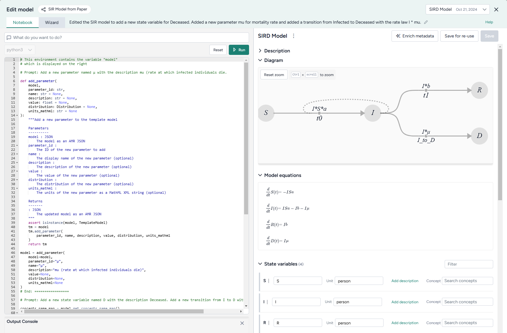
Generated code appears below your prompts, where you can preview, edit, and run it. Each prompt and response builds on the previous ones, letting you gradually make complex changes and save the history of your work.
Note
Each new prompt and response adds new code below any existing code. When you run the Edit model operator, all the code is executed, not just your latest changes.
Open the Edit model code notebook
- Make sure you've connected a model or model configuration to the Edit model operator and then click Open.
Use the AI assistant to edit a model
The Edit model AI assistant interprets plain language to answer questions about or transform your model.
Tip
The AI assistant can perform more than one command at a time.
Ask the AI assistant a question about your model or the process of editing
- Click in the text box at the top of the page, enter your question, and then click Submit .
- Click Show thoughts to view the answer.
Edit a model using the AI assistant
- Click in the text box at the top of the page and then perform one of the following actions:
- Select a suggested prompt and modify it to fit your model and required edits.
- Enter a plain-language description of the changes you want to make.
- Click Submit to generate and preview the model edit code.
- Review and edit (if necessary) the generated model edit code.
- Click Run.
Add or edit code
At any time, you can edit the code generated by the AI assistant or enter your own custom code.
Add or make changes to model edit code
- Directly edit the python code.
- Click Run.
- If needed, review any errors in the Output Console below the code.
Write initials, observables, and rate laws as expressions
In addition to setting initials, observables, and rate laws as numeric values, you can define them as expressions involving other states or parameters. Expressions should follow SymPy syntax. They can include:
-
Elementary operators (
*./,+,-, and**).Example
(S + I + R) ** (1/2) -
Mathematical and logical operations for symbolic-to-numeric computation.
Example
log(Pi + 1e-9, 10) * exp(-t) + Max(-10, Pi * t)
Example
t = sympy.Symbol('t')
EV_i_t_raw, EV_min, EV_max = sympy.Symbol('EV_i_t_raw EV_min EV_max')

model.observables['NewObs'] = Observable(
    name = 'NewObs',
    expression = SympyExprStr((sympy.log(EV_i_t_raw * 1e9, 10) - sympy.log(EV_min * 1e9, 10) / (sympy.log(EV_i_t_raw * 1e9, 10) - sympy.log(EV_max * 1e9, 10))))
Edit model examples
The following sections show examples of how to prompt the Edit model AI assistant to perform commonly used edits.
Add observables by pattern
For a stratified model, you can add observables by pattern. For example, with a model stratified by age (children, adults, elderly) and vaccination status (vaccinated, unvaccinated]:
Add an observable called susceptible_vaccinated_children for the susceptible identifier and for vaccinated children
Expand an equation
You can use the Edit model operator to take a high-level equation and progressively expand it by substituting definitions of variables into the equation. By doing this in multiple iterative steps over several connected Edit model operators, you can create a fully detailed model with clear relationships and dependencies.
Replace rate law t1 with the equation i * s * omega * (1 - (1/e)**(theta * IR**2 * Cv * Ci * IR * Vdrop * tContact / ((AER + lambda + S) * Vair)))
Save an edited model
Each time you click Run, Terarium creates a new edited model as the output for the Edit model operator. This lets you return to previous versions of your model or choose the best one to save and use in your workflow.
When you're done making changes, you can connect the chosen output to any operators in the same workflow that take models as an input.
To use an edited model in other workflows, save it as a project resource.
Choose a different output for the Edit model operator
- Use the Select an output dropdown.
Save an edited model to your project resources
You can save an edited model at any time.
- (Optional) If you created multiple outputs during your edits, Select an output to save.
- Click Save for re-use, enter a unique name in the text box, and then click Save.
Download an edited model
- Click > Download.
Stratify a model
You can make a simple model more complex by stratifying its state variables and parameters. Stratification builds many different versions of a model and its parameters—by location, demographics, or other contextual data—into one large model. You can then configure, calibrate, or simulate the combined models all at once.
Note
For more examples and information about model stratification, see the MIRA training material.
Stratify model operator
In a workflow, the Stratify model operator takes a model as an input and outputs a stratified version of the model.
Tip
For complex stratification schemes, it can be helpful to chain several Stratify model operators together. To make the generated matrices easier to understand, use as many parameters as the number of stratification levels.
Once you've completed the stratification, the thumbnail preview shows the updated model diagram.
Add the Stratify model operator to a workflow
- Perform one of the following actions:
- On a resource or operator that outputs a model or a model configuration, hover over the output and click Link > Stratify model.
- Right-click anywhere on the workflow graph, select Modeling > Stratify model, and then connect a model or model configuration to the input.
Stratify a model
The Stratify model operator adapts to your level of coding experience. You can stratify a model using:
- A wizard view with the most common settings.
- A code notebook with an interactive AI assistant.
Open the Stratify model operator
- Make sure you've connected a model or model configuration to the Stratify model operator and then click Open.
Use the wizard to stratify a model
Use the wizard view of the Stratify model operator to quickly apply commonly used stratification settings. Simply choose:
- The name of your strata.
- The variables and parameters you want to stratify.
- A list of labels for each group.
- Whether to allow interactions and transitions between strata.
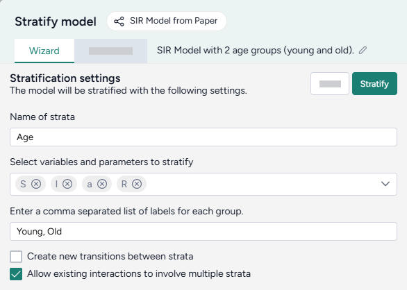
Choose what and how to stratify
-
Enter a name for the strata you want to add.
Note
If you choose to save the stratified model for re-use, the text you enter here becomes part of the suggested model name.
-
Select the model variables and parameters you want to stratify.
Tip
Only stratify the parameters that differ for each stratum.
-
Enter a comma-separated list of labels for each of the strata groups.
Young, Old, MiddleAgedLabels are added to the selected variables and parameters for stratification, with an underscore
_separating them (S_Young). -
Choose whether to allow interactions and transitions between strata.
Stratify the model
- Once you have completed all the settings, click Stratify.
Tip
Strata group labels should only contain letters (a–Z) and numbers (0–9). Don't use special characters like +, -, \, /, or *.
- Recommended:
0to17, 18to65, 66plus - Not recommended:
0-17, 18-65, 66+
Because strata labels become part of mathematical symbols, they must adhere to SymPy naming conventions.
Allow transitions and interactions between strata
You can configure transitions and interactions in stratified models to customize dynamics between groups, such as age or location categories.
Example: interactions and transitions between strata in an SIR model
The following image shows how the transition and interaction settings apply to a simple SIR model stratified by y, m, and o:
- Black lines are the base model. Stratification essentially creates a copy of it for each of the three strata.
-
Blue lines show interactions between strata (Allow existing interactions to involve multiple strata). The susceptible group in each stratum can interact with the infected groups from all strata.
For example were this an age model, a susceptible young person could become infected after interacting with an infected older adult.
-
Red and green lines show transitions between strata (Create transitions between strata).
For example were this a location model, a susceptible person could travel between location o and m.
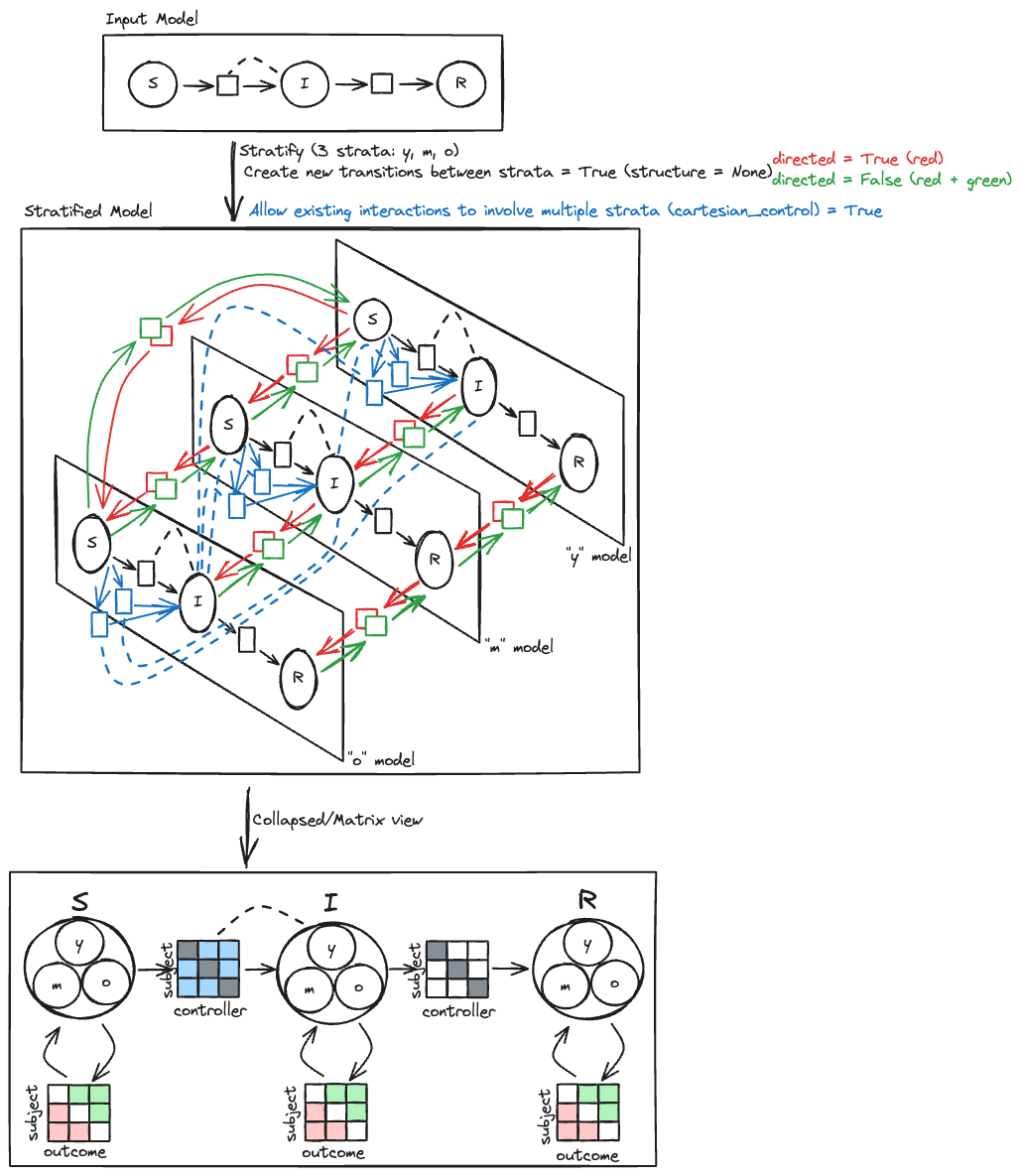
Create transitions between strata
Select Create transitions between strata when you want the strata to be able to transition between each other. For example, when stratifying by:
- Age, this option is usually off because people don't change age groups. (A susceptible young person can't become a susceptible older adult).
- Location, this option can be:
- On if people can travel between locations. (A susceptible person in one county can move to another).
- Off if people are quarantined or social distancing. (A susceptible person in Canada can't travel to the U.S. due to border restrictions).
For more control over which strata can transition and which cannot, see the code notebook.
Allow existing interactions to involve multiple strata
Select Allow existing interactions to involve multiple strata when you want the strata to be able to interact with each other across existing interactions. For example:
- When stratifying an SIR model by age, turn this option on to allow the age groups in each state to interact with age groups in other states.
Use the notebook to stratify a model
In the notebook, you can prompt the AI assistant to:
- Answer questions about the model or stratification options.
- Make more complicated stratifications than possible with the wizard.
You can edit anything the assistant creates or add your own custom code.
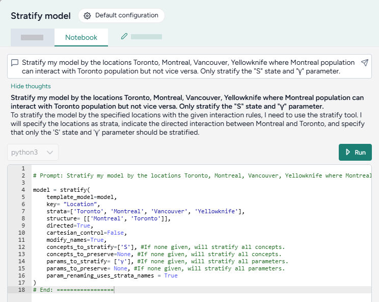
Open the Stratify model notebook
- Click Notebook.
Prompt the AI assistant to stratify a model
The Stratify model AI assistant interprets plain language to answer questions about or stratify your model.
Tip
The AI assistant can perform more than one command at a time.
Ask the AI assistant a question about your model or the process of stratification
- Click in the text box at the top of the page, enter your question, and then click Submit .
- Click Show thoughts to view the answer.
Prompt the AI assistant to stratify your model
- Click in the text box at the top of the page and then perform one of the following actions:
- Select a suggested prompt and edit it to fit your model and the stratification you want to make.
- Describe the stratification you want to make.
- Click Submit .
- Review and edit (if necessary) the generated stratification code.
- Click Run.
Add or edit code
At any time, you can edit the code generated by the AI assistant or enter your own custom code.
The notebook environment uses a structured data format to represent stratification operations. You can edit the code to have greater control over the transitions, interactions, and naming conventions for the stratified model.
model = stratify(
    template_model=model,
    key= "Age",
    strata=['Young', 'Old'],
    structure= [],
    directed=False,
    cartesian_control=True,
    modify_names=True,
    concepts_to_stratify=['S', 'I', 'E', 'H', 'R', 'D'], #If none given, will stratify all concepts.
    concepts_to_preserve=None, #If none given, will stratify all concepts.
    params_to_stratify= None, #If none given, will stratify all parameters.
    params_to_preserve= None, #If none given, will stratify all parameters.
    param_renaming_uses_strata_names = True
)
Stratification code settings
| Setting | Description |
|---|---|
|
key (Name of strata setting in Wizard) |
The characteristic along which the model should be divided, such as age, location, vaccination status. |
| strata | Groups into which the model should be divided. If the key is "Age", strata might be ['young', 'middle-aged', 'old']. |
|
structure (Create new transitions between strata setting in Wizard) |
Pairs of strata within the same state that can interact with each other. For example, ['young', 'old'] allows the 'young' stratum to interact with the 'old' stratum. If no structure is specified, all strata can interact with each other. |
| directed |
Controls the flow of effects or interactions within the model. Useful in scenarios where the direction of interaction matters, such as disease transmission or information flow.
|
|
cartesian_control (Allow existing interactions to involve multiple strata setting in Wizard) |
Determines whether strata from different state variables can interact with each other.
|
| modify_names |
Determines whether the names of states in the model should be altered to include the strata names.
|
|
concepts_to_stratify (Controlled by Variables and parameters to stratify setting in Wizard) |
List of the state variables to stratify. |
| concepts_to_preserve | List of the state variables that shouldn't be stratified. |
|
parameters_to_stratify (Controlled by Variables and parameters to stratify setting in Wizard) |
List of the parameters to stratify. |
| parameters_to_preserve | List of the parameters that shouldn't be stratified. |
| param_renaming_uses_strata_names |
Determines whether the names of parameters in the model should be altered to include the strata names.
|
Add or make changes to stratification code
- Directly edit the python code.
- Click Run.
Examples of AI-assisted stratifications
The following examples show how to prompt the Stratify model AI assistant to perform commonly used stratifications.
Stratify all state variables and parameters
To stratify all the state variables and parameters in the SIR model by age, simply list the strata you want to divide them into.
Stratify my model by the ages young, middle, and old
model = stratify(
    template_model=model,
    key= "Age",
    strata=['young', 'middle', 'old'],
    structure= [],
    directed=False,
    cartesian_control=False,
    modify_names=True,
    concepts_to_stratify=None, # Stratify all concepts.
    concepts_to_preserve=None, # Stratify all concepts.
    params_to_stratify= None, # Stratify all parameters.
    params_to_preserve= None, # Stratify all parameters.
    param_renaming_uses_strata_names = True
)
Stratify with full interaction
Stratify the model by city, and then enable susceptible individuals from each stratum (city) to interact with infected individuals from every other city.
Stratify my model by the locations Toronto, Montreal, Vancouver, Yellowknife where all populations can interact with each other
model = stratify(
    template_model=model,
    key= "Location",
    strata=['Toronto', 'Montreal', 'Vancouver', 'Yellowknife'],
    structure= [],
    directed=False,
    cartesian_control=True, # Allow interactions across different strata
    modify_names=True,
    concepts_to_stratify=None,
    concepts_to_preserve=None,
    params_to_stratify= None,
    params_to_preserve= None,
    param_renaming_uses_strata_names = True
)
Stratify without interaction
Stratify the model by age, but don't allow susceptible individuals in a stratum (age group) to interact with infected individuals from other age groups.
Stratify my model by the ages young, middle, and old. Assume that the age groups cannot interact.
model = stratify(
    template_model=model,
    key= "Age",
    strata=['young', 'middle', 'old'],
    structure= [],
    directed=False,
    cartesian_control=False, # Restrict interactions across different strata
    modify_names=True,
    concepts_to_stratify=None,
    concepts_to_preserve=None,
    params_to_stratify= None,
    params_to_preserve= None,
    param_renaming_uses_strata_names = True
)
Stratify with asymmetric interaction
Stratify the model by city, but only allow individuals from Montreal to interact with individuals from Toronto.
Stratify my model by the locations Toronto, Montreal, Vancouver, Yellowknife where Montreal population can interact with Toronto population but not vice versa
model = stratify(
    template_model=model,
    key= "Location",
    strata=['Toronto', 'Montreal', 'Vancouver', 'Yellowknife'],
    structure= [['Montreal', 'Toronto']], # Allow Montreal and Toronto to interact
    directed=True, # Allow interactions from Montreal to Toronto but not Toronto to Montreal
    cartesian_control=False,
    modify_names=True,
    concepts_to_stratify=None,
    concepts_to_preserve=None,
    params_to_stratify= None,
    params_to_preserve= None,
    param_renaming_uses_strata_names = True
)
Choose which states and parameters to stratify
Stratify only the susceptible state and γ parameter by city.
Stratify my model by the locations Toronto, Montreal, Vancouver. Only stratify the "S" state and "γ" parameter.
model = stratify(
    template_model=model,
    key= "Location",
    strata=['Toronto', 'Montreal', 'Vancouver'],
    structure= [],
    directed=False,
    cartesian_control=False,
    modify_names=True,
    concepts_to_stratify=['S'], # Only stratify the susceptible state
    concepts_to_preserve=None,
    params_to_stratify= ['γ'], # Only stratify the y parameter.
    params_to_preserve= None,
    param_renaming_uses_strata_names = True
)
Exclude states and parameters from stratification
Stratify every state and parameter by city except infected and the β parameter.
Stratify my model by the locations Toronto, Montreal, Vancouver, Yellowknife. Do not stratify the "I" state and "β" parameter.
model = stratify(
    template_model=model,
    key= "Location",
    strata=['Toronto', 'Montreal', 'Vancouver', 'Yellowknife'],
    structure= [],
    directed=False,
    cartesian_control=False,
    modify_names=True,
    concepts_to_stratify=None,
    concepts_to_preserve=['I'], # Stratify all states except infected.
    params_to_stratify= None,
    params_to_preserve= ['β'], # Stratify all parameters except β.
    param_renaming_uses_strata_names = True
)
Answer a question about parameter settings
Ask the AI assistant to explain your model structure and give more details about stratification settings.
What is cartesian_control in stratify?
Cartesian control in the context of stratifying a model determines whether strata from different state variables can interact with each other. If set to true, it allows for interactions across different strata, meaning that entities from one stratum (e.g., infected individuals in one location) can interact with entities in another stratum (e.g., susceptible individuals in another location). If set to false, it restricts interactions such that entities from different strata cannot interact, isolating the dynamics within each stratum.
Interpret the stratified model
Terarium previews the stratified model as:
- A color-coded diagram that shows the base model and the newly added strata.
- A list of stratified state variables, parameters, observables, and transitions.
When reviewing the stratified model, you can get a sense of the state variables and parameters in the list below the diagram, but the results are easiest to understand in matrix form.
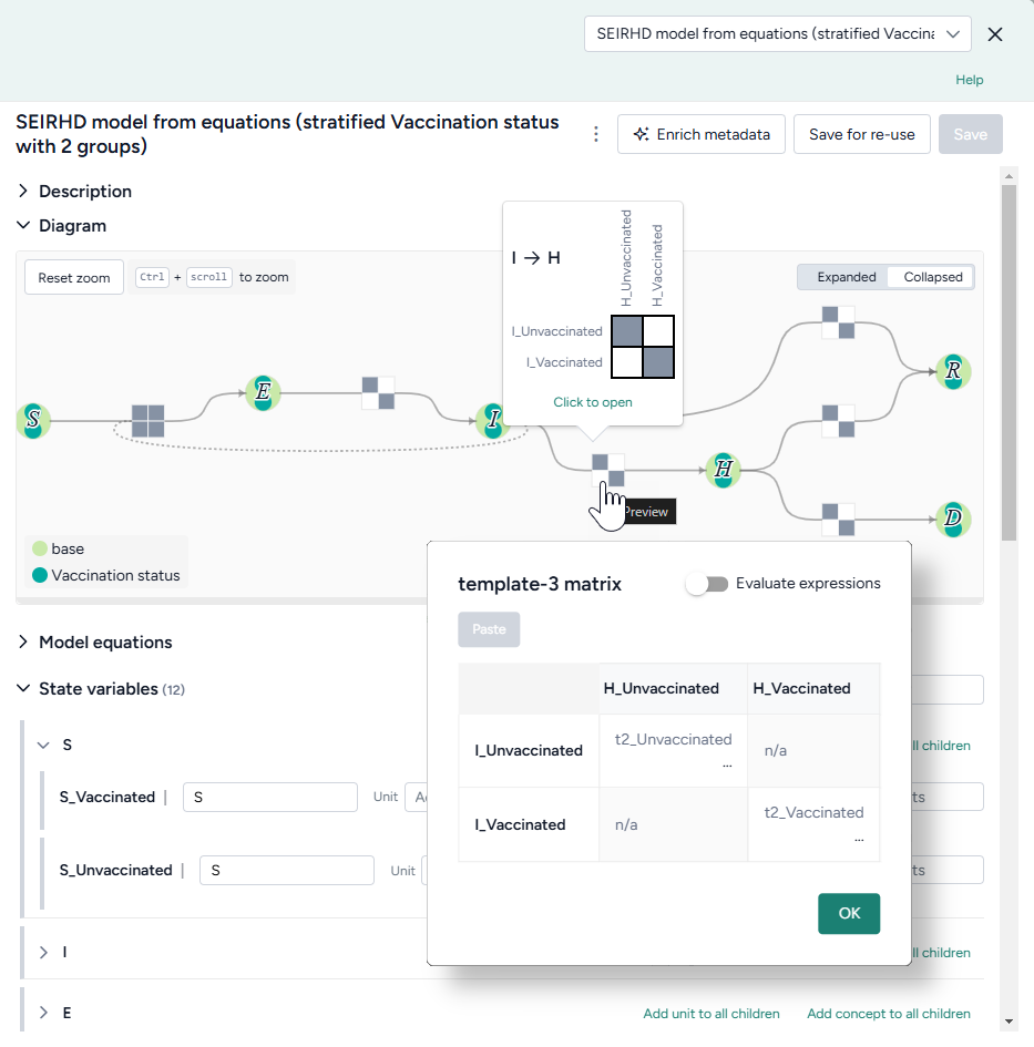
Review stratified state variables or parameters
In the model diagram:
- Hover over a transition matrix to see how the different strata interact. Grey cells show that the corresponding strata can interact.
- Click the matrix to see the equations that describe the interactions.
In the list of state variables, parameters, observables, and transitions, perform one of the following actions:
- Click Preview next to a symbol name.
-
Click Open matrix.
Note
For parameter matrices, use the dropdown to select the type of interactions you want to view:
- subjectOutcome: Parameters for the relationship between the subject (the entity undergoing change) and the outcome (the result of that change).
- subjectControllers: Parameters for how controllers (external entities involved in the process) influence the subject (the entity undergoing change).
- outcomeControllers: Parameters for how controllers (external entities involved in the process) influence the outcome (the result of that change). The controller does not experience the outcome but facilitates the transition.
- other: Factors or intermediary states other than subjects, controllers, or outcomes that affect the process.
The block matrices in the model diagram should hint at the collapsed transitions.
Save a stratified model
Saved models appear in your Resources panel and as the output of the Stratify model operator.
Save a stratified model as a new model in Terarium
You can save your stratified model as a new model at any time.
- Click Save for re-use, edit the name of the stratified model, and then click Save.
Download a stratified model
- In the Output panel, click > Download.
Compare models
You can compare two or more models in Terarium to see:
- A brief overview of their structural and metadata similarities and differences.
- Side-by-side comparisons of key model details.
- An AI-assisted visualization of common and unique state variables and transitions across each model.
The Compare models operator is powered by an interactive AI assistant. The assistant automatically compares the models based on any enriched metadata and can generate summaries tailored to your modeling goals.
Compare models operator
In a workflow, the Compare models operator takes two or more models as inputs and shows side-by-side comparisons of them. It does not output any data for use in other operators.
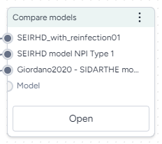
-
Inputs
Two or more models
-
Outputs
N/A
Add the Compare models operator to a workflow
-
Perform one of the following actions:
- On a resource or operator that outputs a model, click Link > Compare models.
- Right-click anywhere on the workflow graph, select Modeling > Compare models, and then connect the output of two or more models to the Compare models inputs.
Get model comparisons
The Compare model operator has a wizard view and a code notebook:
- The wizard view provides AI-generated text summaries of model similarities and differences.
- The code notebook allows you to create a visual comparison that shows the similarities and differences between the models.
Use the wizard to compare models
The wizard view compares the selected models along the following lines. For the best results, make sure you've enriched each model before running the comparison.
Create a goal-driven comparison overview
The goal-driven model comparison overview highlights the similarities and differences between the selected models. An AI assistant generates the overview by reviewing and summarizing the following structural and metadata components of the models.
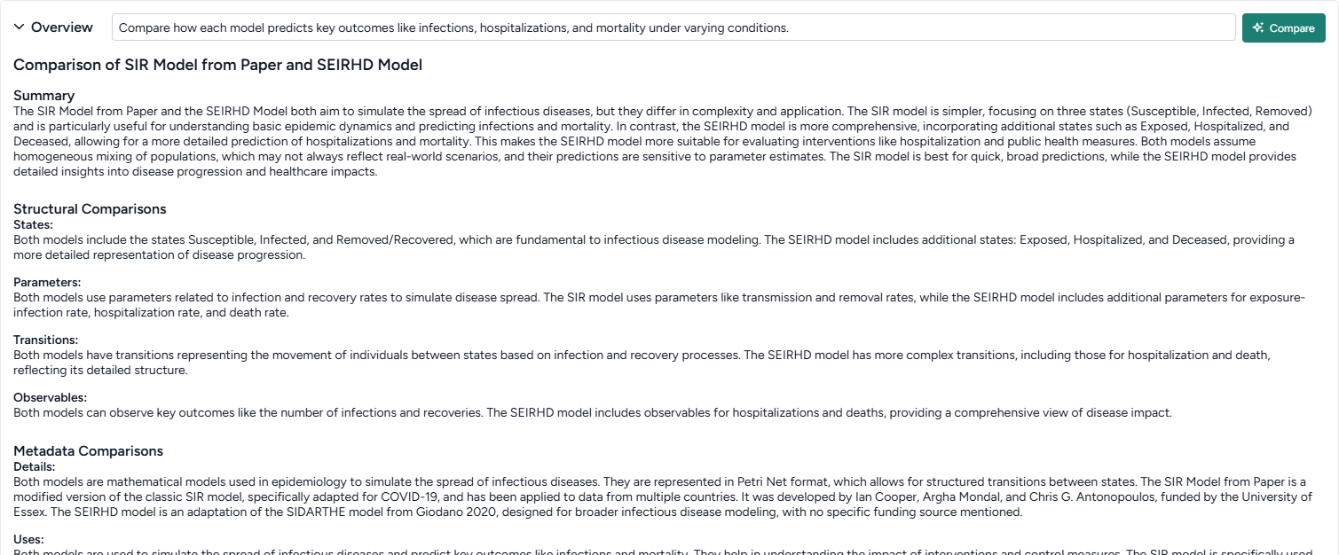
Note
- Before generating the overview, you can specify your goal for comparing the models. The assistant then produces the overview summary with your goal as context.
- Metadata comparison is only available if you've first enriched the selected models.
-
Summary
A high-level comparison of the models, highlighting their strengths, weaknesses, and intended use cases. If you provide a goal, the summary incorporates it to ensure the analysis aligns with your specific focus.
-
-
Structural Comparison
This section compares the structures of each model.
- States: Compares the state variables across models, focusing on similarities and differences in names, descriptions, and initial conditions.
- Transitions: Highlights similarities and differences in transitions, including input/output states and mathematical expressions.
- Parameters: Examines shared and unique parameters, detailing names, values, and usage in rate laws.
- Observables: Summarizes observables, comparing names, IDs, and expressions across models.
-
Metadata Comparison
This section is only available if you've enriched the selected models.
- Details: Summarizes common and unique metadata, such as source, authorship, funding, and model type.
- Uses: Discusses shared and unique contexts for using each model, including direct, indirect, and potential misuse scenarios.
- Biases, Risks, and Limitations: Identifies common and unique biases, risks, and limitations, with a focus on assumptions, potential harms, and mitigations.
- Testing and Validation: Compares evaluation protocols, testing data, and metrics, highlighting fairness, privacy, and other social considerations.
Get an AI-generated analysis of the models related to your goals
- Enter your goal for comparing the models and click Compare.
Get side-by-side model card comparisons
The side-by-side model cards let you visually compare the following key aspects of the selected models. The model cards are based on an AI summary of their underlying metadata.
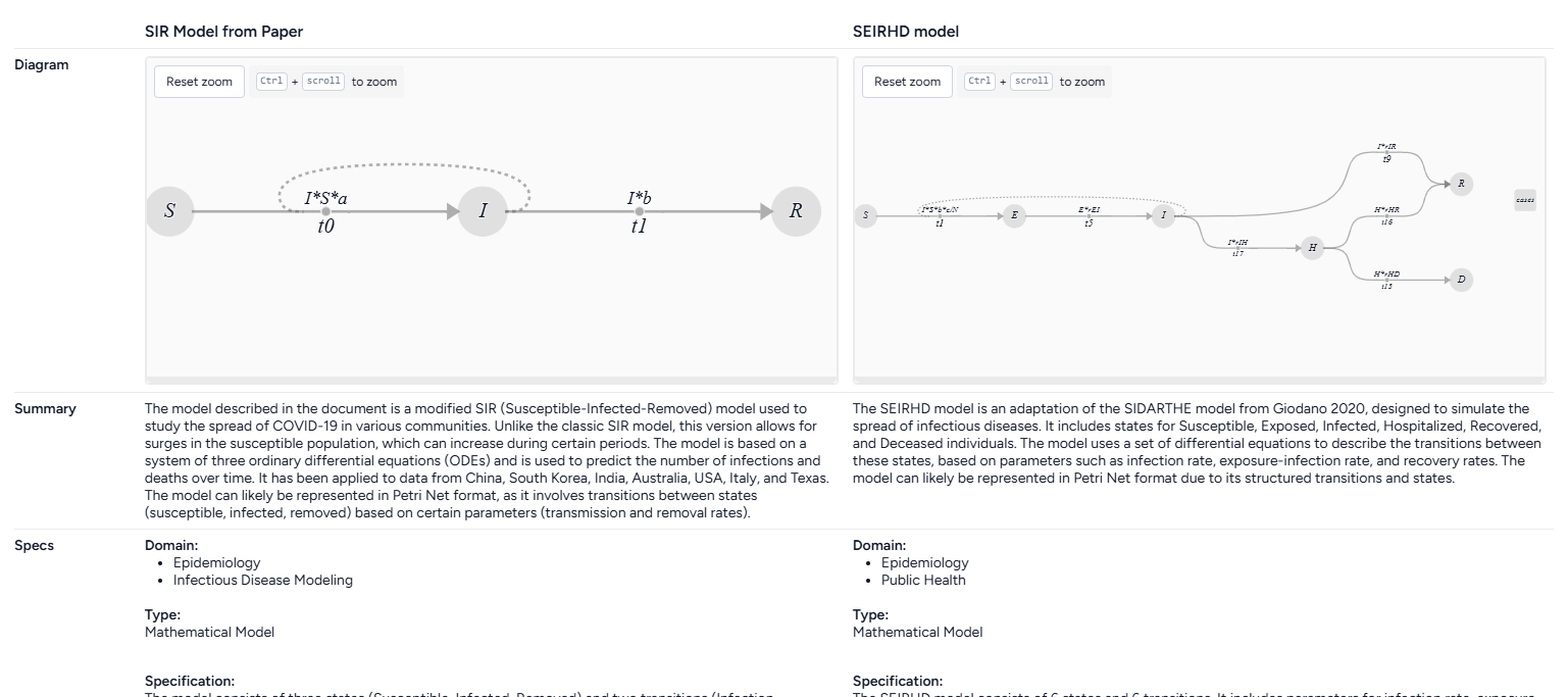
Note
Model cards are only available if you've first enriched the selected models. Otherwise, the model cards only show the model name and diagram.
-
Model name
-
Model diagram
-
Summary
A description of the model, how it is intended to be used, and whether it can be represented in Petri Net format.
-
Specs
- Domain: Areas where the model is relevant or can be effectively utilized.
- Type: How the model is represented, Mathematical Model, Graphical Model, or Other.
- Specification: Detail about the model's structure and complexity, including the number of places, transitions, parameters, and arcs.
- States: A list summarizing the model states, including what they represent, their initial values, their units, and how they can transition to other states.
- Parameters: A list summarizing the model parameters, including what they represent, their units, and how they influence transition rates.
-
Uses
- Direct use: How the model can be used to analyze or simulate real-world scenarios.
- Out of scope use: Instances where using the model would be inappropriate or misleading.
-
Bias risks limitations
- Biases: Factors that may skew the model's outputs or affect its accuracy.
- Risks: Potential issues that could compromise the model's reliability or safety.
- Limitations: Constraints that define the model's scope or performance boundaries.
-
Testing
- Validation: How the model was validated, such as through simulation or comparison with real-world data.
- Metrics: Criteria used to assess the model's performance.
-
Getting started
Instructions or examples on how to use the model.
-
Glossary
A list of terms and definitions.
-
Authors
A list of authors of the model.
-
Citation
A list of citations relevant to the model.
-
More information
- Funded by: Funding sources.
- Links: Links to additional information about the model.
Get aside-by-side model card comparisons
- Make sure you've enriched each model before opening the Compare models operator.
Review model concept comparisons
The concept comparisons highlight the relationships and differences between the concepts and states in the models. The comparison is presented in following formats to visualize the refinements and equivalences between concepts and identify how the models approach similar ideas.
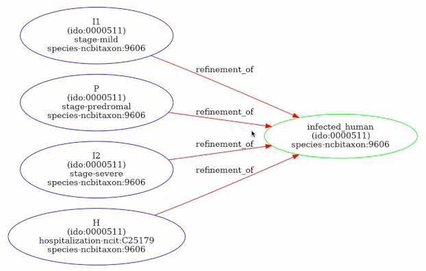
Note
- Concept comparison is available only if you've enriched the selected models.
-
Concept context comparison
A list of concepts in the models and how often they appear in each one.
-
-
Tabular concept comparison
A table that compares the concept relationships between states in two models:
=: The concepts behind the states are equivalent.<: The concepts in the state on the left are a subset or a more specific instance of the concepts in the state on the top.>: The concepts in the state on the left is a superset or a more general instance of the concepts in the state on the top.- Blank: The concepts are not equal.
-
Concept graph comparison
A graph showing how the model states and concepts are related, highlighting refinements and equivalences.
Each node is a state or concept. The color shows the model it belongs to:
- Blue: From the first model.
- Green: From the second model.
- Orange: Shared by both models.
Edges between nodes represent refinement relationships or equality between concepts. For refinement relationships, the direction of the arrow shows that the source is a refinement of the target.
Use the notebook to visually compare models
The AI assistant in the Compare models operator can visualize the similarities and differences of the attached models. It creates a comparison diagram for every pair of input models. The diagram is color-coded to show the state variables and transitions that are unique to each model and common to both.
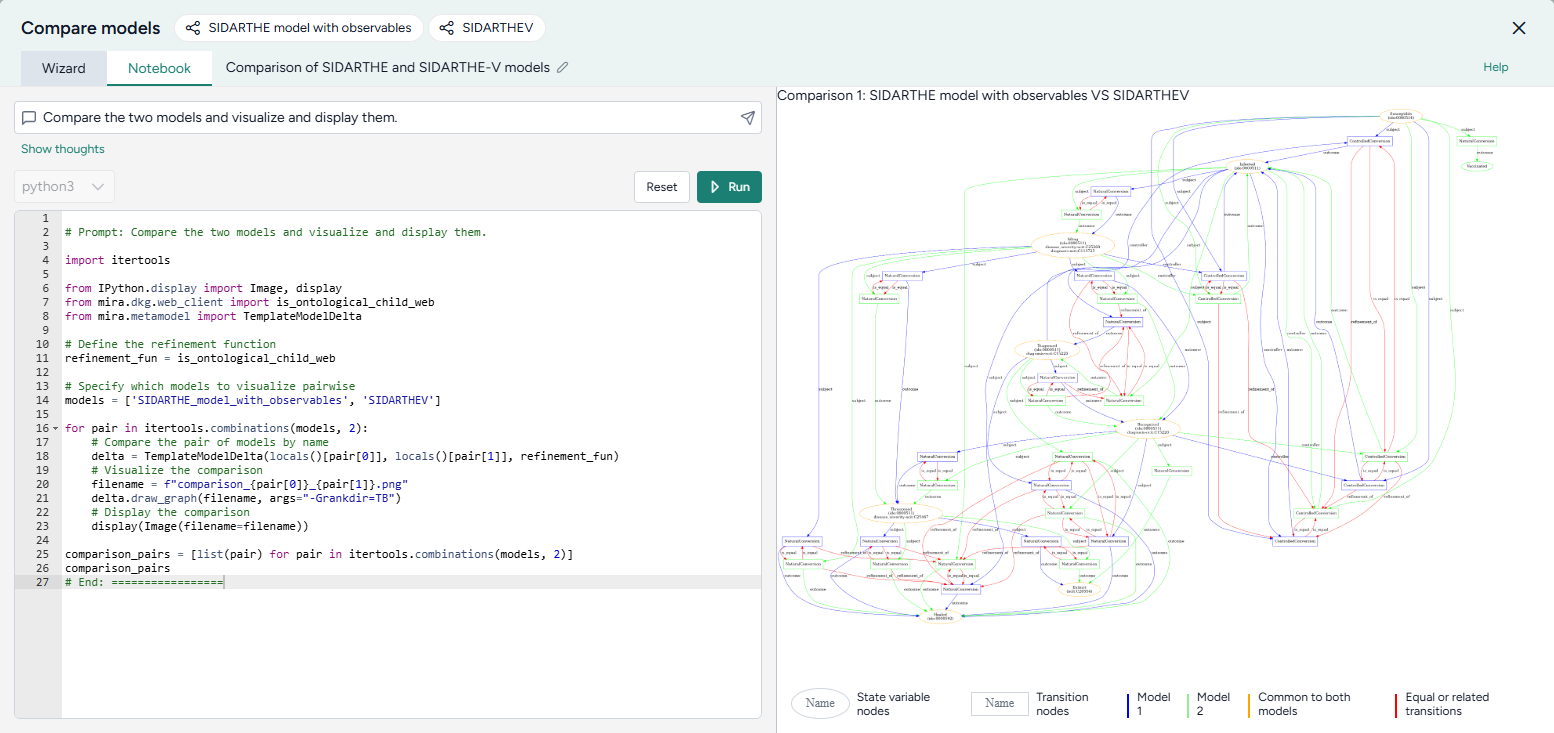
Visualize model similarities and differences
- Click Notebook.
- Click in the prompt field, select Compare the models and visualize and display them, and then click Submit .
- Review the generated code and then click Run.
- Review the model diagrams in the Preview.
- To make changes, modify the selected prompt or the generated code and click Run again.
Ended: Modeling
Configuration and intervention ↵
Configuration and intervention
With Terarium's configuration and intervention operators, you can:
-
Set initial values and parameters to prepare your model for simulations and analyses.
-
Validate a model configuration
Make sure your model configuration is accurate by checking for errors such as changing population values, violations of non-negativity, and other custom constraints.
-
Define strategies or actions to influence your model's behavior under specific conditions.
-
Optimize an intervention policy
Fine-tune your intervention strategies to achieve the best possible outcomes.
-
Simulate an intervention policy
Assess the impact of your intervention on a variable of interest.
Configure a model
Before running a simulation, you need to configure your model by setting the initial values and parameters for the condition you want to test. You can use the Configure model operator to:
- Automatically extract a configuration from an optional document or dataset.
- Manually enter values and account for uncertainty in any downstream simulations.
- Select from previously saved configurations in the current project.
Configure model operator
In a workflow, the Configure model operator takes a model as an input and outputs a model configuration. You can also input an optional document or dataset (such as a contact matrix or initial populations) from which to automatically extract variable and parameter values.
Once you have selected a configuration, the operator in the workflow shows its name and description.
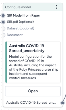
Add the Configure model from equations operator to a workflow
-
Do one of the following actions:
- On a resource or operator that outputs a model, click Link > Configure model.
- Right-click on the workflow graph, select Config & Intervention > Configure model, and then connect the output of a model to the Configure model input.
-
If needed, connect the output of a Document or Dataset to the Configure model inputs.
Configure a model
Configuring a model tailors it to meet the requirements of your simulations, calibrations, and analyses. The Configure model operator adapts to your level of coding experience. You can configure a model using:
- A wizard view with the most common settings.
- A code notebook with an interactive AI assistant.
Open the Configure model operator
- Make sure you've connected a model to the Configure model operator and then click Open.
Edit the name and description of a configuration
To help you understand your workflow at a glance, the name and description of the selected model configuration appear on the Configure model operator in the notebook. You can update these in the wizard to provide more context.
- To change the title, click Edit , enter a unique name, and press Enter.
-
To change the description:
- Click Expand to expand the Description section if necessary.
- Click Edit , enter a unique name, and then click Apply .
- Click Save.
Use the wizard to configure a model
Use the wizard view of the Configure model operator to:
- Extract a configuration from project resources.
- Select from previously saved configurations.
- Manually enter or edit configurations.
Extract a model configuration from a document or dataset
You can use the wizard to automatically attempt to extract variable and parameter values from any attached documents or datasets.
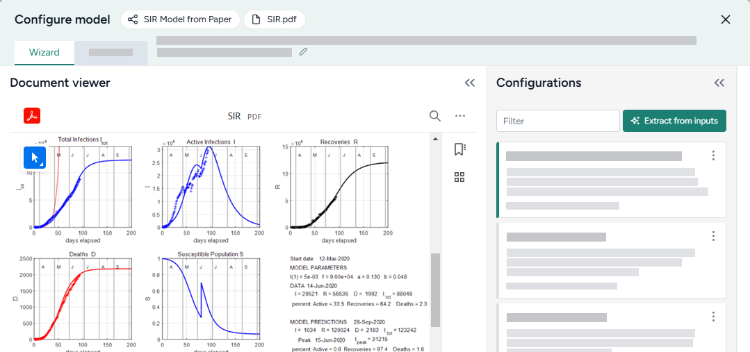
Extract a configuration from a document or dataset
- Click Extract from inputs.
- Review and edit any of the extracted initial or parameter values as needed.
Choose an existing model configuration
Each time you create a configuration for a model, Terarium saves it to your project. Whenever you add or edit a Configure model operator, you can quickly select any of the existing configurations.
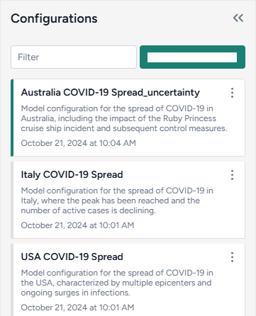
Search the available model configurations
- In the Configurations panel, use the Filter field to search for keywords in configuration names and descriptions.
Choose an existing model configuration
- Review the Configurations on the left. Click a configuration name to select it and review its values.
- Close the Configure model wizard.
Edit or create a model configuration
When you edit or create a model configuration, you can set a start date for its timeline, customize initial state and values, and apply uncertainty.
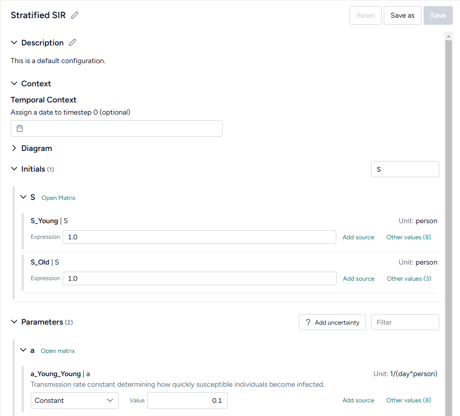
Tip
- The card for the selected configuration in the Configurations panel shows if any of the initials or parameters are missing values. Review this before you finish your configuration to make sure you don't miss anything.
- To manually copy configuration values from an attached document, click Expand to expand the Document viewer so you can review the paper while making your updates.
Set a start date for the model's timeline
Tip
Before setting the start date for the model, make sure you've edited the model metadata to specify the units (days, months, or years) for each timestep.
If your model includes a time component, you can assign a date to the starting timestep (0). This allows you to view and select start and end dates in downstream simulations, calibrations, or interventions.
- Click inside the Date field and choose a start date from the calendar.
Search the model states and parameters
-
Click inside the Filter field for Initials or Parameters and type the name of the state or parameter you're looking for.
Note
The filter works only with original, unstratified state and parameter names. To find a stratified state or parameter, search using the name of the original state or parameter it was derived from.
Edit the initial value of a model state
You can edit the initial values of model state variables either as numeric values or as expressions involving other states or parameters.
-
If your state variable is stratified, click Expand to show the stratified states.
Tip
To set all the stratified variables at once, copy a range of values from a spreadsheet, click Open matrix, and then click Paste.
-
Do one of the following actions:
- Enter a numeric value or a SymPy expression in the Expression field.
- Click Other values, select a value from another model configuration, and then click Apply selected value.
-
(Optional) Click Add source and enter an explanation for how or why you came up with the value.
Edit the value of a parameter
-
If your parameter is stratified, click Expand to show the stratified parameters.
Tip
To set all the stratified parameters at once, copy a range of values from a spreadsheet, click Open matrix, and then click Paste.
-
Choose the type of value to enter:
- To enter a single unchanging value, select Constant and enter the value.
- To enter a range of possible values, select Uniform and enter the minimum and maximum possible values.
- Alternatively, click Other values, select a value from another model configuration, and then click Apply selected value.
-
(Optional) Click Add source and enter an explanation for how or why you came up with the value.
Add uncertainty to parameters
You can quickly add uncertainty to all or some of your parameters with constant values.
- Click Add uncertainty.
- Enter a percentage value for the uncertainty range. For example, if the parameter's value is
1and you set the uncertainty to10%, the parameter becomes a uniform distribution between0.9(Min) and1.1(Max). -
Select the parameters that you want to apply uncertainty to and then click Apply.
Note
You cannot apply uncertainty to parameters that are already uniform distributions.
Write initial values as expressions
In addition to setting the initial values of model state variables as numeric values, you can define them as expressions involving other states or parameters. Initials written as expressions should follow SymPy syntax. They can include:
-
Elementary operators (
*./,+,-, and**).Example
(S + I + R) ** (1/2) -
Mathematical and logical operations for symbolic-to-numeric computation. Simply call the functions by removing the
sympy.prefix.Example
log(Pi + 1e-9, 10) * exp(-t) + Max(-10, Pi * t)
Note
In the wizard view, only the initials support SymPy expressions. You can add SymPy expressions for initials, observables, and rate laws in the notebook view.
Use the notebook to configure a model
In the notebook, you can prompt an AI assistant to:
- Describe the model's configuration
- Modify parameters, initial conditions, and other attributes of the model.
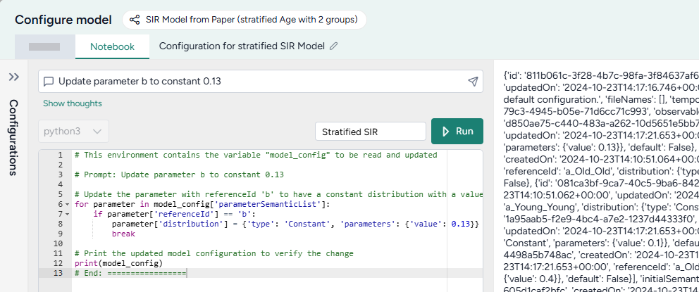
You can edit anything the assistant creates or add your own custom code.
Tip
The assistant can be helpful when you need to set expressions or values that are the product of complicated formulas.
Open the Configure model notebook
- Click Notebook.
Prompt the AI assistant to configure a model
The Configure model AI assistant interprets plain language to answer questions about or stratify your model.
Tip
The AI assistant can perform more than one command at a time.
Ask the AI assistant a question about your model configuration
- Click in the text box at the top of the page, enter your question, and then click Submit .
- Click Show thoughts to view the answer.
Prompt the AI assistant to configure your model
- Click in the text box at the top of the page and then do one of the following actions:
- Select a suggested prompt and edit it to fit your model and the configuration you want to make.
- Describe the configuration you want to make.
- Click Submit .
-
Review and edit (if necessary) the generated configuration code.
Note
In some cases, the AI assistant may ask for clarifying questions before generating code. For example, if you ask to update a stratified parameter by its original name, it may ask if you want to update all the stratified parameters or only one. In these cases, update your prompt as needed and then click Submit again.
-
Click Run.
- Click Wizard and find the modified initials or parameters to verify that they were correctly updated.
Add or edit code
At any time, you can edit the code generated by the AI assistant or enter your own custom code.
Add or make changes to model configuration code
- Directly edit the python code.
- Click Run.
Write initials, observables, and rate laws as expressions
In addition to setting initials, observables, and rate laws as numeric values, you can define them as expressions involving other states or parameters. Expressions should follow SymPy syntax. They can include:
-
Elementary operators (
*./,+,-, and**).Example
(S + I + R) ** (1/2) -
Mathematical and logical operations for symbolic-to-numeric computation.
Example
```python log(Pi + 1e-9, 10) * exp(-t) + Max(-10, Pi * t)
Example
t = sympy.Symbol('t')
EV_i_t_raw, EV_min, EV_max = sympy.Symbol('EV_i_t_raw EV_min EV_max')

model.observables['NewObs'] = Observable(
    name = 'NewObs',
    expression = SympyExprStr((sympy.log(EV_i_t_raw * 1e9, 10) - sympy.log(EV_min * 1e9, 10) / (sympy.log(EV_i_t_raw * 1e9, 10) - sympy.log(EV_max * 1e9, 10))))
Examples of AI-assisted model configurations
The following examples show how to prompt the Configure model AI assistant to make commonly used configurations.
Ask a question about the current model configuration
What are the model parameters and current values?
Set a range of values for a model parameter to account for uncertainty
Update parameter beta to a uniform distribution with max 0.5 and min 0.2
Save a model configuration
By default, any changes you make to initials or parameters are automatically saved to the configuration selected in the Configurations panel. Saved model configurations appear any time you connect the model to a Configure model operator in your project. The selected configuration becomes the output of the Configure model operator.
Save your edits as a new model configuration
- Click Save as.
- Enter a unique name for your configuration and click Save.
Undo your edits
- Click Reset.
Choose a different output for the Configure model operator
- Select a configuration from the Configurations panel.
Download a model configuration
Note
You can import downloaded model configurations into other projects. Doing so recreates the model from which the configuration was derived.
- In the Configurations panel, click > Download.
Use the model configuration output
With the configure model output, you can:
Validate a model configuration
In your modeling workflow, you might have multiple candidate models that contain mistakes and generate unphysical predictions. You can use the Validate configuration operator to check the outputs of these models. In the case of compartmental models, the operator can run the basic check wherein the population of every compartment, for all timepoints, is non-negative and less than or equal to the sum of the initial condition values.
The Validate configuration operator supports several types of constraints you can build to check for additional assumptions on the inputs and outputs of the model:
- "greater/less than or equal to": that a model quantity (state variable, parameter, or observable) be bounded below/above by some threshold value.
- "increasing/decreasing": that the time derivative of a model quantity is positive or negative.
- "linearly constrained": that several parameters satisfy a linear constraint of the form
L ≤ a_1 * p_1 + a_2 * p_2 + ... + a_k * p_k ≤ U. - "following": that a model quantity remains within some range of a given time-series dataset for all given timepoints (not yet supported).
The output of this operator is a new model configuration that represents the largest region in the parameter space (as defined by the input configuration) which satisfies all the given constraints.
Validate configuration is powered by the run_validate function of the Functional Model Analysis (Funman) package.
Example
-
Given a SIR-type compartmental model where the state variables represents relative fraction of a total population, you want to check that:
- All the state variables are greater than zero,
- They are less than one,
- The
S(t)state variable is decreasing monotonically (assuming no births), and - The
R(t)state variable is increasing monotonically (assuming no deaths).
-
Given a model with parameters
β, γ, you want to find what model configuration would satisfy the linear inequalityβ ≤ 2 * γ. You can create a constraint of the form:parameters β, γ should be linearly constrained from timepoint 0 timepoint 30 days with inequality
0 ≤ -1 * β + 2 * γ.The result is a model configuration where the parameters
β, γare uniform distributions, covering a region of parameter space where the inequality is satisfied.
Validate configuration operator
The Validate configuration operator takes a model configuration as an input and returns a validated model configuration as output. The output can be used in simulation operators downstream.
Tip
When setting up the input configuration:
- For each parameter of interest, specify a wide uniform distribution in the input configuration so the Validate configuration operator has a sufficiently large parameter space to search for regions that satisfy all the given constraints.
- You can use the Edit model operator to define observables for quantities that do not correspond to any existing model state variables or parameters.
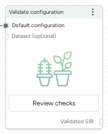
How it works: funman
-
Inputs
- Model configuration
- Dataset (optional)
-
Outputs
Validated model configuration
Add the Validate configuration operator to a workflow
-
Do one of the following actions:
- On an operator that outputs a model configuration, click Link > Validate configuration.
- Right-click anywhere on the workflow graph, select Config & Intervention > Validate configuration, and then connect a model to the Validate configuration input.
Validate a model configuration
The Validate configuration operator allows you to define model checks and produce validated model configurations using:
- A wizard view with the most common settings.
- A notebook view with structured JSON inputs and outputs.
Open the Validate configuration operator
- Make sure you've connected a model configuration to the Validate configuration operator and then click Open.
Use the wizard to validate a model configuration
Use the wizard view of the Validate configuration operator to apply validation settings. You can:
- Include common compartmental constraints.
- Build your own custom constraints.
- Choose how to run the validation.
Use compartmental constraints
Compartmental constraints provide a simple validation layer for your model configuration by enforcing basic physical that make sure:
- The state variables don't become negative for all timepoints.
- The total population of the model are conserved and constant for all timepoints.
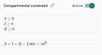
Troubleshooting the compartmental constraint
In the case where the compartmental constraint prevents results from being returned, try defining it as a custom constraint:
-
Prompt the Edit model AI assistant to:
Create an observable that is the sum of all the state variables -
Create a new configuration for the edited model.
-
Add a custom constraint that linearly constrains the new observable above and below the total population.
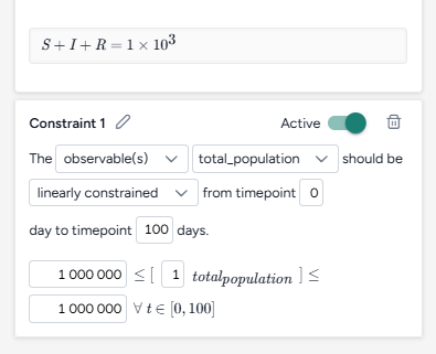
Custom version (bottom) of the compartmental constraint (top) limiting the new observable above and below the total population.
Turn the compartmental constraints on or off
- Turn the Active toggle on or off.
Add a custom constraint
By building custom constraints, you can tailor the validation process to your specific needs. You can constrain state variables, parameters, and observables to adhere to rules or trends critical for your analysis.
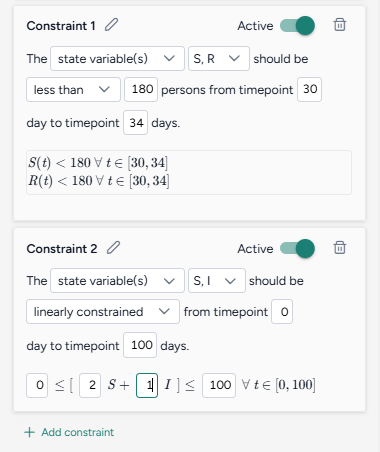
Terarium simplifies the process of building constraints by reducing them to readable sentences from which you select your preferred options. When you're done, the constraint is summarized as one or more mathematical expressions.
Add a constraint
- Click Add constraint.
- Click Edit , enter a unique name, and then click Apply .
Keep a model quantity above or below a value
- Select the type and name of the quantity you want to constrain.
- Select the condition that the quantity should satisfy—less than, less than or equal to, or greater than—and then specify the value.
- Choose the timepoints between which the condition should be enforced.
Keep a model quantity from increasing or decreasing
- Select the type and name of the quantity you want to constrain.
- Select the condition that the quantity should satisfy—increasing or decreasing.
- Choose the timepoints between which the condition should be enforced.
Enforce a linear relationship between model quantitys
- Select the type and name of the quantitys you want to constrain.
-
Select the linearly constrained condition and then in the formula below, enter:
- The weights for each quantity.
- The lower and upper bounds between which the weighted quantitys should stay.
-
Choose the timepoints between which the condition should be enforced.
Turn off a constraint
- Turn the Active toggle off.
Delete a constraint
- Click Delete
Configure the run settings
Run settings let you customize the scope and precision of the validation process. To help you get started, you can choose between fast or precise presets.
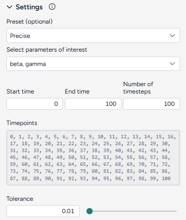
Configure the run settings
- Select a Preset, Fast or Precise, to balance between run time and precision in parameter space and prediction error
-
Select the Parameters of interest. Model checks applied on parameters that are not selected are ignored.
Note
You can only select parameters that are represented by a uniform distribution. Parameters with constant values can't be selected.
-
Choose the Start and End time.
Advanced settings
Using the following advanced settings, you can further optimize the computational efficiency and thoroughness of the validation:
- Number of timesteps: More timesteps provide a detailed view of how the model behaves over time and smaller prediction error, while fewer timesteps simplify the analysis and reduce run time when precision isn't as critical.
-
Tolerance: Controls how finely the operator segments the parameter space for validation. The value is the relative size of the smallest sub-region that will be checked for satisfiability.
1.0means "do not segment the input parameter space at all" while0.1means "segment the space down to 10% of the parameter ranges".Tip
Start with <10 timesteps, a high tolerance (~0.5), and select 2 or 3 parameters of interest for reduced run time; increase the number of timesteps and lower the tolerance towards 0.01 for higher precision and lower prediction error.
Use the notebook to validate a model configuration
The notebook exposes structured JSON that describes the model, its configuration, and the same settings available in the Wizard. You can directly edit the JSON and then run it to create a new validated configuration (also represented as a structured JSON).
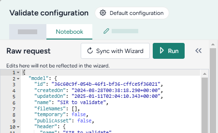
Note
Changes you make to the validation JSON do not automatically copy over to the wizard.
Edit code
- Directly edit the JSON.
Sync code with wizard settings
- Click Sync with Wizard.
Create the validated configuration
Once you've configured the validation settings, you can run the operator to generate a new validate configuration. The new configuration becomes a temporary output for the Validate configuration operator; you can connect it to other operators in the same workflow. If you want to use it in other workflows, you can save it for reuse.
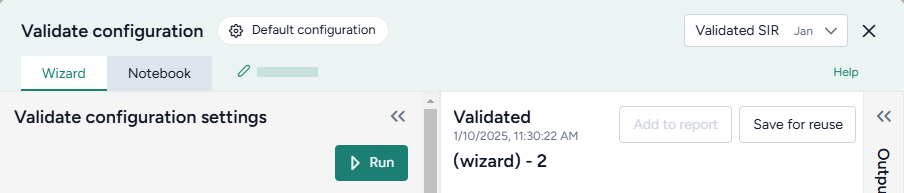
Create a new validate model configuration
-
Click Run.
Tip
The run progress of the Validate configuration operator is displayed in the workflow. Close the operator to view it.
Choose a different output for the Validate configuration operator
- Use the Select an output dropdown.
Save the new configuration for selection in Configure model operators
- Click Save for reuse, enter a unique name for the configuration, and then click Save.
Understand the validation result
The validation result is displayed as a series of plots showing the satisfactory and unsatisfactory state and parameter values over time. The following sections show how to interpret these.
Only show furthest results
When analyzing model behavior, intermediate results can sometimes make it hard to focus on the most comprehensive outcomes. You can instead display only the most extensive calculations performed for each combination of parameter values. This shows the final iteration where the model has computed the farthest timepoint necessary to ensure all checks either pass or fail.
- Click Only show furthest results.
States variables and observables
State variable and observables plots provide a time-series view of how these model quantities evolve over time. The simpler constraints (greater/less than some threshold value) are shown as light blue rectangles. Altogether, the plots show how and when each model quantity visually passes or fails the given constraints. Each trajectory is mapped from a single sampled point in parameter space:
- Dark green lines satisfy all model checks.
- Yellow lines do not satisfy all model checks.
- Light green lines are ambiguous within the precision of the validation.
- Light blue boxes show the constraints you set up.
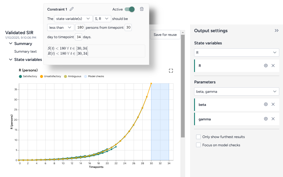

Show or hide state variable or observable plots
- Click Expand to expand the Output settings.
-
Do one of the following actions:
- Use the dropdown to search, select, or clear different variables.
- Click X to remove a variable plot.
Focus on model checks
In some cases, the results of the validation may not approach the constraints you set up. In these instances, the model checks do not appear on the plots. To expand a plot to view the full extent of the model checks:
- Click Expand to expand the Output settings.
- Click Focus on model checks.
Parameter plots
Parameter plots allow you to explore how variations in model parameters influence the outcome of validation checks. These plots highlight which parameter ranges are valid and where constraints are violated:
- Dark green lines satisfy all model checks.
- Yellow lines do not satisfy all model checks.
- Light green lines are ambiguous within the precision of the validation.
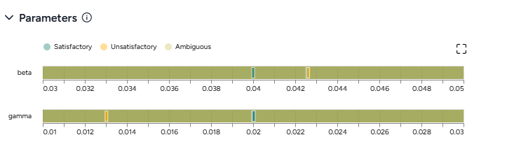
Show or hide parameter plots
- Click Expand to expand the Output settings.
-
Do one of the following actions:
- Use the dropdown to search, select, or clear different parameters.
- Click X to remove a parameter plot.
Only show furthest results
The validation algorithm is efficient and only solves the model ODEs incrementally. It computes outcomes with the minimum timepoints that is necessary to guarantee that all the model checks either pass or fail. These intermediate results can sometimes make it hard to focus on the trajectories that are actually validated. You can instead restrict the plot to only these trajectories by toggling on this option.
- Click Only show furthest results.
Troubleshooting
Long run times
If your validation is taking too long, try reducing the complexity of the validation problem:
- Reduce the number of timesteps to ~5.
- Reduce the number of parameters of interest to two or three of the most important.
- Increase the tolerance to ~0.5.
- Crop out parameter ranges that cause numerical instability. For example, if you have SIR-type model and a recovery rate
γthat is an uniform distribution between-1.0and1.0, the model may become unstable nearγ = 0as the basic reproduction numberR₀ → ∞. You can narrow the distribution ofγto exclude the singularity at the origin.
Following these steps can help you reduce the run time or produce non-trivial validation results.
No satisfactory conditions
If the results contain no satisfactory conditions, it often means the entire parameter range is unsatisfactory. Try running validation again on an input configuration with wider parameter ranges.
Next steps
You can use the new validated configuration in simulations to forecast, analyze, or explore system behavior based on the validated parameters. Validation reduces the need to repeatedly reconfigure a model to find physical starting points for simulations, calibrations, and optimizations.
Create an intervention policy
You can define intervention policies to specify changes in state variables or parameters at specific points in time. This can help you answer key decision-maker questions like:
How does increasing vaccination rate affect cases and hospitalizations?
Create intervention policy operator
In a workflow, the Create intervention policy operator takes a model and an optional document as inputs and outputs an intervention policy.
Once you've created the intervention policy, the thumbnail preview shows brief descriptions of the interventions you set up.
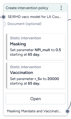
-
Inputs
- Model
- Document (optional)
- Dataset (optional)
-
Outputs
Intervention policy
Add the Create intervention policy operator to a workflow
-
Do one of the following actions:
- On an operator that outputs a model, click Link > Create intervention policy.
- Right-click anywhere on the workflow graph, select Config & intervention > Create intervention policy, and then connect the output of a model to the Create intervention policy inputs.
Create an intervention policy
Use the Create intervention policy operator to:
- Extract an intervention policy from a project resource.
- Select from previously saved interventions.
- Manually edit or create an intervention.
Open the Create intervention policy operator
- Make sure you've connected a model to the Create intervention policy operator and then click Open.
Extract an intervention policy from a project resource
You can automatically attempt to extract intervention policies from any attached documents or datasets.
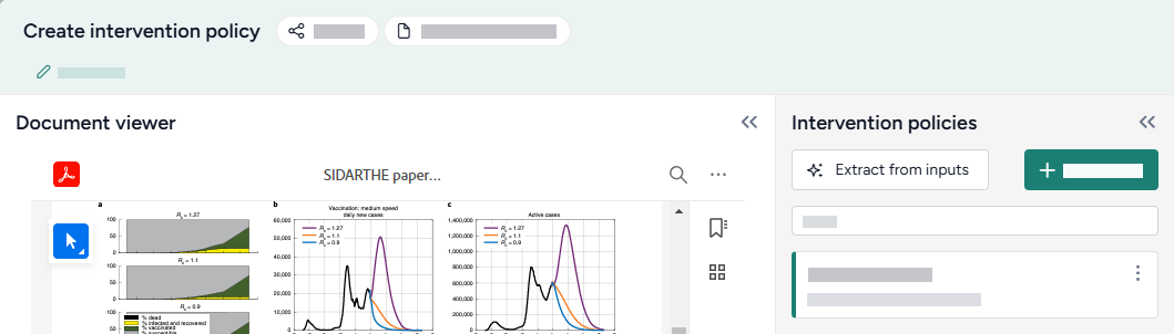
Extract an intervention policy from a document or dataset
- Click Extract from inputs.
- Review and edit any of the extracted intervention policy settings as needed.
Choose an existing intervention
Each time you create an intervention for a model, Terarium saves it to your project. Whenever you add or edit a Create intervention policy operator, you can quickly select any of the existing interventions.
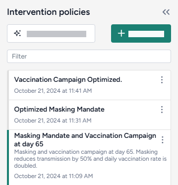
Search the available intervention policies
- In the Intervention policies panel, use the Filter field to search for keywords in intervention policy names and descriptions.
Choose an existing intervention policy
- Review the Intervention policies on the left. Click a intervention policy name to select it and review its values.
- Close the Create intervention policy operator.
Edit or create an intervention
Terarium simplifies the process of building interventions by reducing them to readable sentences from which you select your preferred options. As you select the policy settings, the Output panel visualizes your changes on a chart.
You can create:
- Static interventions that take place at a fixed point in time (start masking in one week).
-
Dynamic interventions that trigger based on conditions such as when state variables cross a threshold (start masking when hospitalizations exceed 5,000).
Note
Dynamic interventions take place the first time the trigger state crosses the selected threshold—whether it's crossing from above or below.
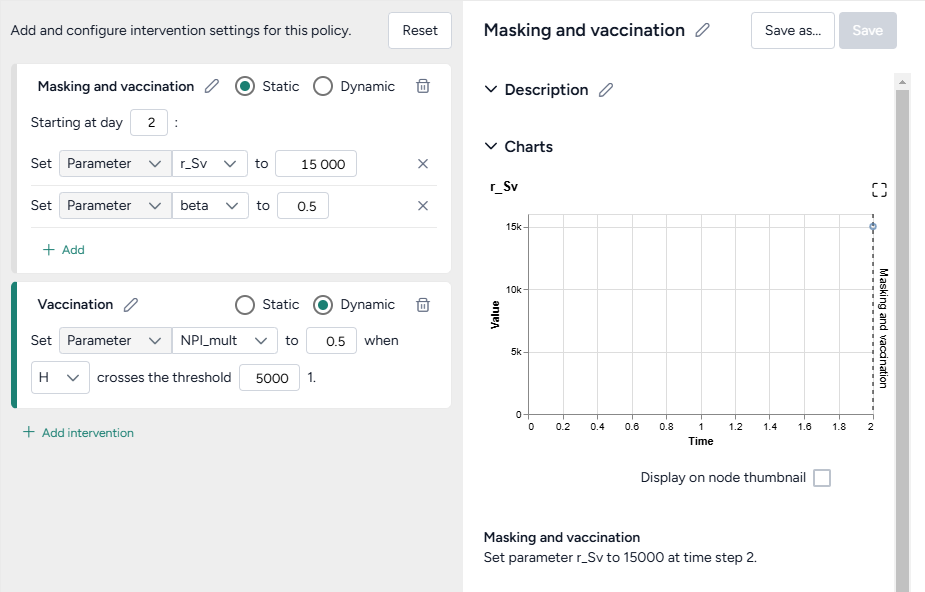
Add a new intervention
- Click Create new.
- Click Add intervention.
- Click Edit , enter a unique name, and then click Apply .
Set up a static intervention
A static intervention sets a parameter or state to a specific value at a specific time. You can add multiple static interventions to start on a given day.
- Select the Static checkbox.
- Enter the starting day timestep to specify when the intervention should begin.
- Select the type and name of the parameter or state variable you want to change.
- Enter a new value for the parameter or state variable.
- (Optional) To change another parameter or variable at the same time, click Add and then repeat steps 2–4.
- Review the charts in the Output panel to verify your policy is set up correctly.
Set up a dynamic intervention
A dynamic intervention sets a parameter or state to a specific value when a state crosses a specific threshold.
- Select the Dynamic checkbox.
- Select the type and name of the parameter or state variable you want to change.
- Enter a new value for the parameter or state variable.
- Select the state and enter the value that should trigger the change.
- Review the charts in the Output panel to verify your policy is set up correctly.
Preview an intervention policy chart on the Create intervention policy operator in the workflow graph
- Select Display on node thumbnail.
Save an intervention policy
By default, any changes you make are automatically applied to the output of the Create intervention policy operator. You can also save intervention policies so they appear any time you connect the model to a Create intervention policy in your project.
Save your edits to the selected intervention policy
- Click Save.
Save your edits as a new intervention policy
- Click Save as.
- Enter a unique name and click Save.
Undo your edits
- Click Reset.
Choose a different output for the Create intervention policy operator
- Select an intervention policy from the Intervention policies panel.
Optimize an intervention policy
Given a model configuration and a proposed intervention policy, you can identify the optimal parameter values and/or times to implement an intervention that satisfy specified constraints. This helps you make informed decisions when faced with questions like:
What is the smallest possible transmission rate reduction that will keep infections below 1000 over the next 100 days?
When is the latest possible time an intervention that reduces the transmission rate by half may be implemented in order to ensure infections remain below 1000 over the next 100 days?
What is the minimal reduction in transmission rate, and the latest time it can be applied in order to keep infections below 1000 over the next 100 days?
Note
In addition to this help, you can find more examples and information about intervention policy optimization in:
Create an optimize intervention policy operator
Assuming you have a model configuration and an intervention policy in your workflow, add an Optimize intervention policy operator:
- Right-click the workflow and select Simulation > Optimize intervention policy.
- Connect your model configuration and proposed intervention policy as inputs.
The output of the Optimize intervention policy operator is an optimized intervention policy.
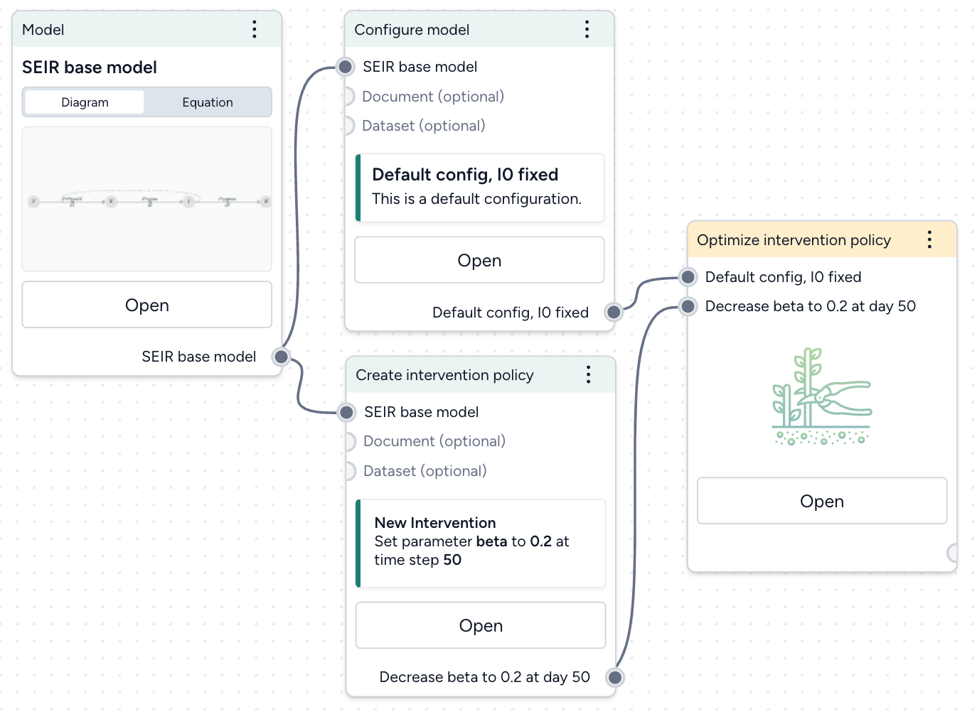
Set your success criteria
Select a threshold and tolerance for simulated outcomes from the dropdowns.
Ensure A is B a threshold of C at D in E% of simulated outcomes.
- A: State variable or observable from your model.
- B: Should the selected state variable remain above or below the threshold?
- C: Threshold value for the chosen state variable.
- D: Time period of interest, should the threshold constraint be met for all timepoints or is it only required for the end of the simulation at the last timepoint?
- E: Risk tolerance as the percentage of simulated trajectories for which the threshold constraint must be met to adopt the intervention policy.
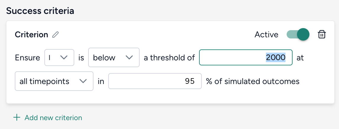
Select how to optimize the intervention policy
Choose which aspects of your intervention policy to optimize and how. Provide an initial guess along with minimum and maximum values to guide your optimization. Adjust the relative importance to create a weighted objective function when there are multiple parameters or start times being optimized.
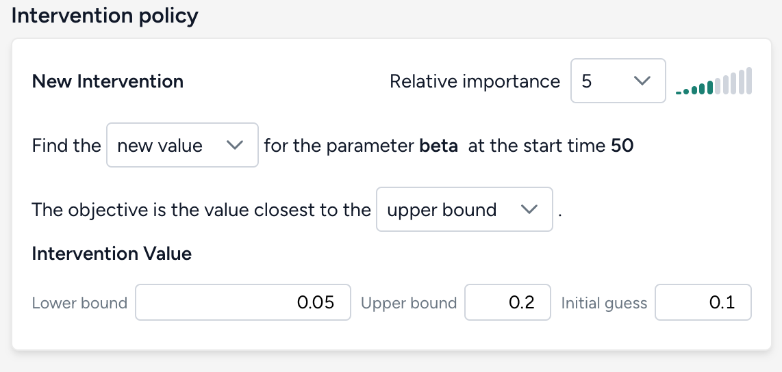
There are three possible targets for optimization.
Parameter value
Find the new value for the parameter parameter in intervention policy at the start time time of intervention in policy. The objective is the value closest to the initial guess, lower bound, or upper bound.
Intervention start time
Find the new start time for the parameter parameter in intervention policy when the value is value in intervention policy. The objective is the initial guess, lower bound, or upper bound start time.
Note
Start timeandEnd timeshould be interpreted as the lower bound and upper bound of the time when the intervention is applied, respectively.- If your goal is to find the latest time an intervention could be implemented and still satisfy the constraint, make your objective the value closest to the upper bound.
Intervention start time and parameter value
Find the new value and start time for the parameter parameter in intervention policy. The objective is the value closest to the initial guess, lower bound, or upper bound and at the initial guess, lower bound, or upper bound start time.
Choose your optimization settings
Choose the duration of your simulation. Advanced settings let you specify how many sample trajectories to run, the differential equation solver method, and the optimizer optiopns.
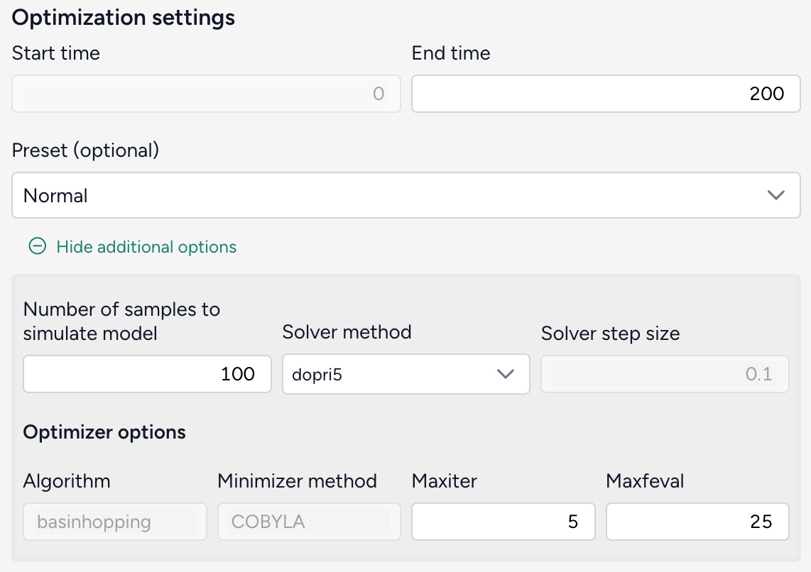
Configure the run settings
- Set the End time to specify the duration of simulation. The Start time always begins at time t = 0.
- Choose a Preset. The default recommended setting is
Normal, which uses thedopri5solver.Fastuses theeulermethod.
Advanced settings
- Number of samples: Each simulation draws this number of samples from the model distribution. Select the number of samples to use. The default value of 100 is great for testing and understanding whether the given optimization will work. Higher values like 1,000 samples give more accurate results and a better sense of uncertainty in the model.
-
Solver method: The default differential equation solver is
dopri5, an adaptive step-size, 5th-order explicit Runge-Kutta method. Theeulerandrk4methods require you to also specify the Solver step size.Note
For the best balance of speed and accuracy, the
rk4ordopri5solver method is recommended. -
Optimizer options
- Algorithm: SciPy
basinhoppingalgorithm. - Minimizer method:
COBYLAis the chosen minimization method used in the basinhopping algorithm. - Maxiter: The maximum number of iterations used in the basinhopping algorithm. Increasing
Maxiterexplores the parameter space more thoroughly and better avoids getting trapped in local minima, but will take longer to run. - Maxfeval: The maximum number of times the optimization function is evaluated during each iteration of the basinhopping process. Increasing
Maxfevalmay improve accuracy, but also increases computation time.
- Algorithm: SciPy
Run the optimization
Once you've configured all the optimization settings, click Run. When the optimization completes, you can view and compare the results of your model simulations with and without the optimized intervention.
A successful optimization looks like this:
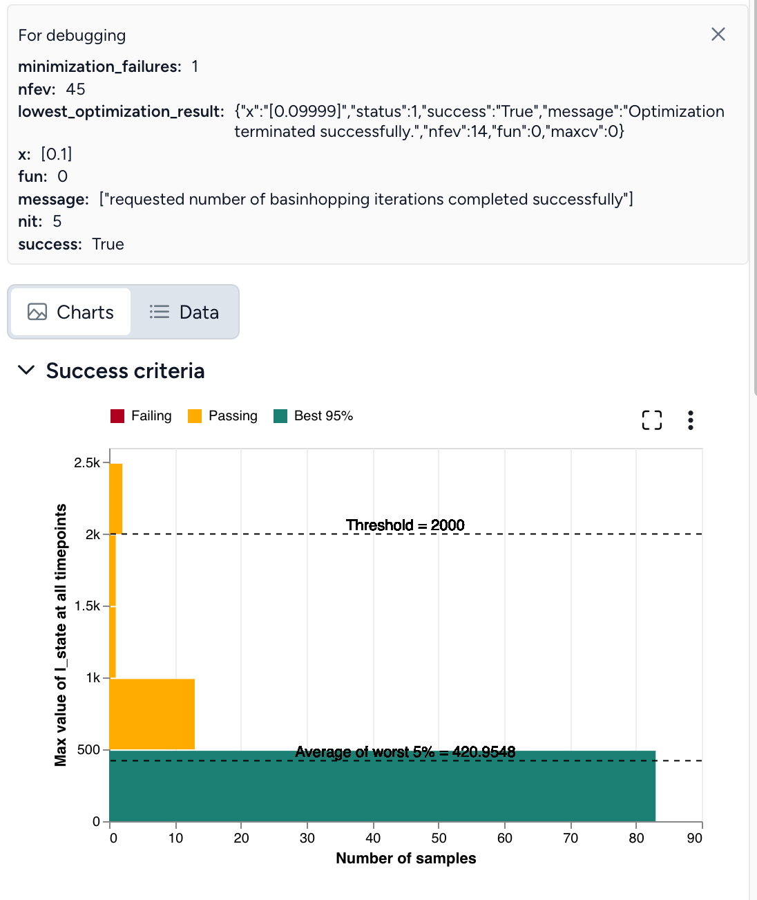
If the optimization does not complete successfully (as shown below), you need to adjust your settings.
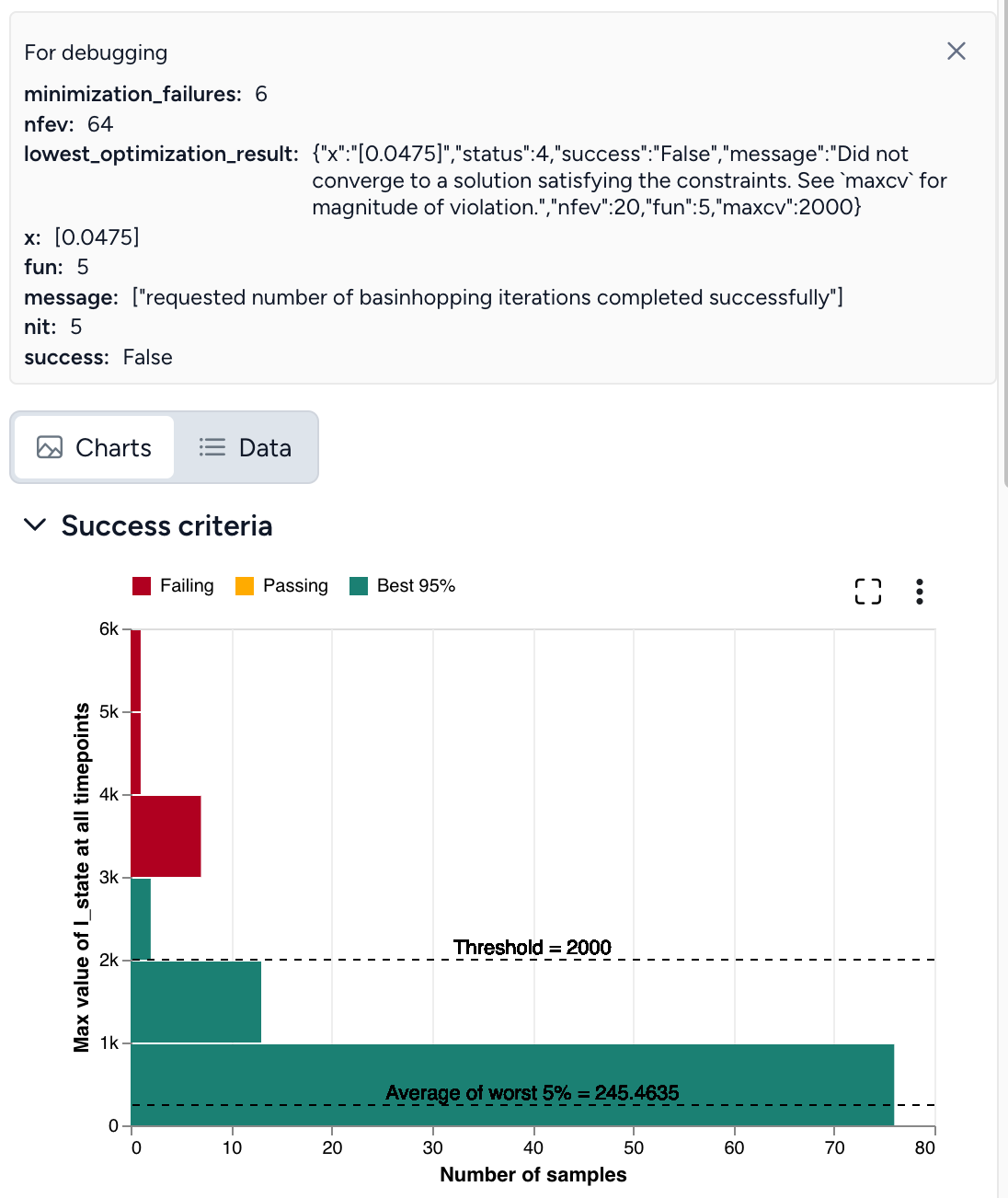
Troubleshooting a failed optimization
Intervention policy optimization is extremely complex. The following tips describe reasons why your optimization may fail and how get a successful optimization. When you encounter failures, repeat as necessary and try combinations of these tips.
Optimal intervention policy is out of bounds
If the optimal intervention policy is out of bounds, try:
- Expanding the bounds for your intervention policy.
- Using a different initial guess for the interventions.
Optimization not satisfying set constraints
lowest_optimization_result: message: Did not converge to a solution satisfying the constraints. See maxcv for magnitude of violation
This error message means that the optimizer didn't find a feasible solution within the bounds for the interventions, the risk bound is too strict to satisfy, or the optimizer ran out of resources (stopped too early).
To address this:
- Check if the threshold value is appropriate for given problem.
- Use a different initial guess for the interventions.
- Increase Maxiter and Maxfeval to provide more time for the optimizer to converge.
- Increase the Number of samples to improve accuracy of Monte Carlo risk estimation.
Seeing yellow
If the results of your optimization look close to successful but aren't quite there yet:
- Rerun the simulation with the intervention set to the optimal value and an increased Number of samples.
- Increase Maxiter and Maxfeval.
Double check your inputs
- Does your model configuration have the correct parameter values and initial states? Are the distributions around your uncertain parameters reasonable or too large?
- As a check, remove or tighten unnecessary sources of uncertainty. For example, if the default configuration of a SEIR model includes substantial uncertainty in the initial infectious population, try setting a fixed number of infectious individuals initially. This can help you investigate how changing the transmission rate impacts infections and discover a successful optimization.
- Is the proposed intervention policy correct? Does the parameter you are intervening have the intended effect on the state variable of interest?
Simulate the model with your proposed intervention applied as a check and compare the results: Thicker solid lines represent the mean trajectory of the simulations, while the optimization focuses on "worst case scenarios" defined by your risk tolerance. Even if the peak of the intervened simulations is close to your desired threshold value, the range of all simulations (shown in lighter gray or green) can be much wider. Asking that the threshold not be exceeded in 95% of simulations is different than it might appear, as the mean being close to the threshold doesn't fully account for the variability, as shown below.
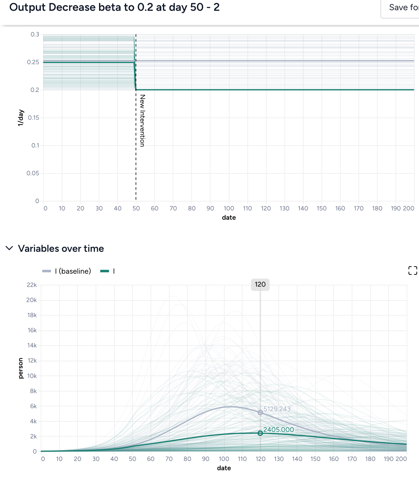
Adjust your threshold
Is the threshold too low or too high? It may be preferable to have a higher threshold if you can be more certain it will not be exceeded.
Adjust your risk tolerance
Depending on the situation, it might be okay for infections to remain below a certain threshold only 75% of the time. But if the threshold for hospitalizations is the number of available beds, it may not be appropriate to become more risk tolerant.
Reassess the bounds of your intervention value or time.
Are the bounds:
- Reasonable? If the lower bound of your parameter is zero, try using a lower bound like 0.01 or 0.001 instead.
- Too restrictive?
- Not restrictive enough? If you want to search a wide swath of the parameter space, consider increasing the number of basinhopping iterations (Maxiter). This gives you more chances to find the global minima of your objective function.
Simulate an intervention policy
You can simulate an intervention policy to assess the impact of your intervention on a variable of interest. For example, you can see how increasing vaccination rate affects hospitalizations.
Build an intervention policy simulation workflow
You can build a workflow to simulate an intervention policy manually.
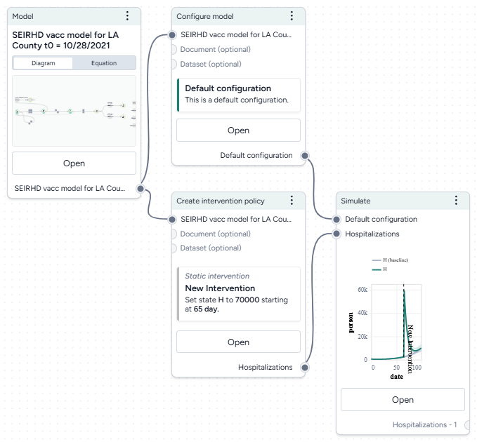
Before you get started, you'll need a:
Once you've set up and run the workflow, you'll have a set of intervention policy simulation results, which you can use as a dataset.
Build an intervention policy simulation workflow
- Add your model to a workflow, hover over its output, and click Link > Configure model. Click Open on the Configure model operator to select or create a new configuration.
- Hover over the Model output again and click Link > Create intervention policy. Click Open on the Create intervention policy operator to select or create a new intervention policy.
- Hover over the Create intervention policy output and click Link > Simulate.
- Click the output of the Configure model operator and connect it to the Simulate model configuration input.
- Connect the model configuration output to the simulate input.
Run a simulation
Once you've built your workflow, you can edit the Simulate run and output settings to generate the intervention policy simulation.
Run an intervention policy simulation
- Click Open on the Simulate operator.
- Select the Simulate run settings.
- Click Run to start the simulation.
- Preview the intervention policy results. To add variables or parameters, use the Output settings.
View and save simulation results with interventions
Simulation results are summarized on the operator in the workflow and in the operator details. When you simulate with an intervention you can see the impacts of the intervention. There are visual representations of:
-
The parameter you changed in your intervention.
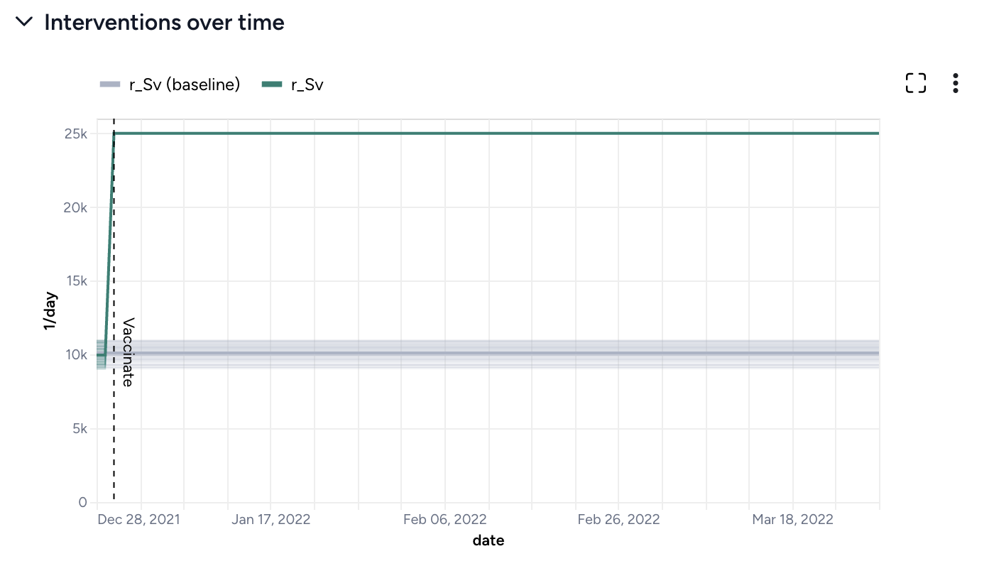
At day 2, vaccination rate increases from 10,000 people per day to 25,000 people per day. -
Simulation results with the intervention shown in green and results for the baseline (no intervention) in gray.
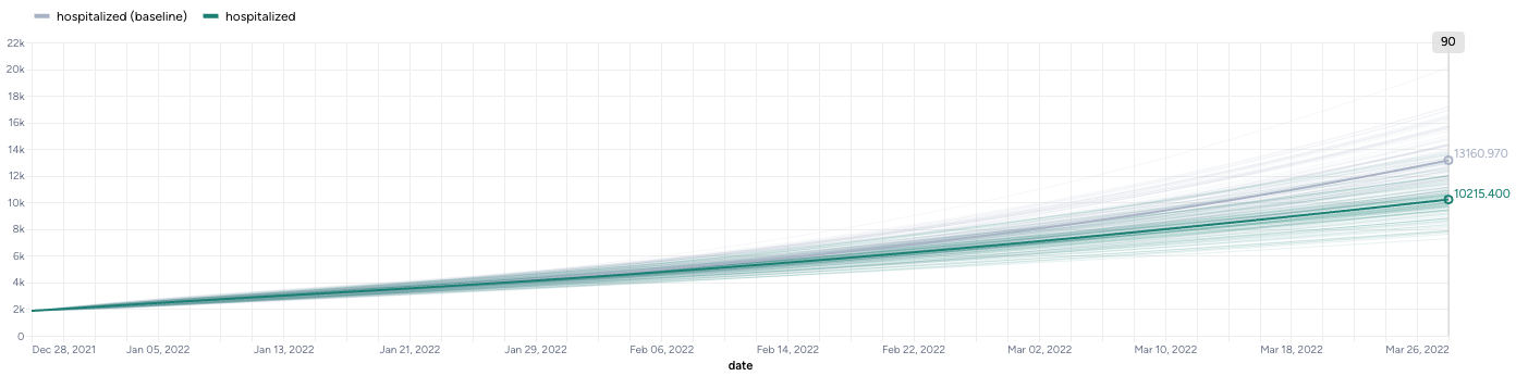
Increasing vaccination rate from 10,000 people per day to 25,000 people per day decreases hospitalization rate from ~13,000 to ~10,000.
Save the simulation results as a new dataset
-
On the Output panel, click Save for re-use.
Tip
Using a descriptive naming convention for your datasets will help you keep track of them when you want to compare multiple scenarios.
Troubleshooting
If the simulation fails and shows an AssertionError: underflow in dt 0.0 error, the configuration has made the model unsolvable with the selected solver Method. This often happens with the dopri5 solver method.
Workaround: Try using a different solver method, such as rk4 or euler. These solvers are be less efficient than dopri5, but they are also less likely to get caught in an unworkable state
Ended: Configuration and intervention
Simulation ↵
Simulation
With Terarium's simulation operators, you can:
-
Understand how the underlying system might behave under specific conditions
-
Determine how changes in model parameters affect the outcome variables of interest.
-
Improve the performance of a model by updating the value of configuration parameters.
-
More info coming soon.
-
Calibrate with multiple models simultaneously to explore how different configurations collectively align with historical data.
Simulate a model
Simulating a model lets you understand how the underlying system might behave under specific conditions.
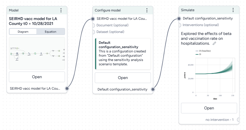
Tip
Simulate early with a simple model. Using a model with a population of 1,000, for example, can help you spot issues and fix them before you incorporate more complexity.
Simulate operator
In a workflow, the Simulate operator takes a model configuration and an optional intervention as inputs. Based on a customizable number of samples (to account for uncertainty) it outputs a set of simulation data.
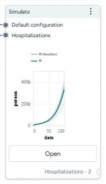
-
Inputs
- Model configuration
- Intervention policies (optional)
-
Outputs
Simulation data
Add a Simulate operator to a workflow
-
Do one of the following actions:
- On an operator that outputs a model configuration or intervention policy, click Link > Simulate.
- Right-click anywhere on the workflow graph, select Simulation > Simulate, and then connect a model configuration to the Simulate input.
Simulate a model
The Simulate run settings allow you to fine-tune the time frame and solver behavior. By adjusting these settings, you can balance performance and precision.
Open a Simulate operator
- Make sure you've connected a model configuration to the Simulate operator.
- Click Open.
Configure the run settings
- Select a Preset, Fast or Normal.
-
Choose the End time to specify the simulation time range.
Note
If you included a starting timestep in your model configuration, the start and end dates also appear in your simulation.
Advanced settings
Using the following advanced settings, you can further optimize the computational efficiency and thoroughness of the simulation:
- Number of samples: Number of stochastic samples to generate.
-
Number of timepoints: Number of data points to generate over the simulation. Use this setting when you want to generate more timepoints than the duration of the simulation.
For example, a simulation with a duration of 10 days has 10 timepoints by default. Use this setting to increase or decrease the number of timepoints generated during the simulation.
-
Method: How to solve ordinary differential equations, dopri5 , rk4, or euler .
Tip
Using a low number of samples and the dopri5 method can speed up your runtime for debugging purposes.
Run the simulation
Once you've configured all the simulation settings, you can run the operator to generate a new simulation results dataset. The new dataset becomes a temporary output for the Simulate operator; you can connect it to other operators in the same workflow. If you want to use it in other workflows, you can save it for reuse.
Create a new simulation run
- Click Run.
Choose a different output for the Simulate operator
- Use the Select an output dropdown.
Save simulation results as a new dataset
- On the Simulate pane, click Save as new dataset.
View simulation results
When the simulation is complete, Terarium shows the results on the operator in the workflow and in the operator details. Available details include:
- An AI-generated description.
- Configurable charts.
- Data table of results.
AI-generated summaries of results
AI-generated summaries of simulation results describe:
- The simulation settings you selected.
- Trends in model parameters and states over time.
- The effects of any interventions on outcomes.
Edit the auto-generated summary
You can edit the summary to provide your own interpretation of the data.
- Click anywhere on the description, make your changes, and press Enter.
Charts
Configurable charts provide a visual way to understand and validate simulation results, allowing you to view interventions over time, compare variables and model states, and perform sensitivity analysis to see how parameter changes affect outcomes.
-
Interventions over time
These charts are only available if you connected an intervention policy to the Simulate input. For more information, see Simulate an intervention policy.
At day 2, vaccination rate increases from 10,000 people per day to 25,000 people per day. -
Variables over time
To aid visual validation, the variables over time charts compare the effects of simulation for state variables and observables.
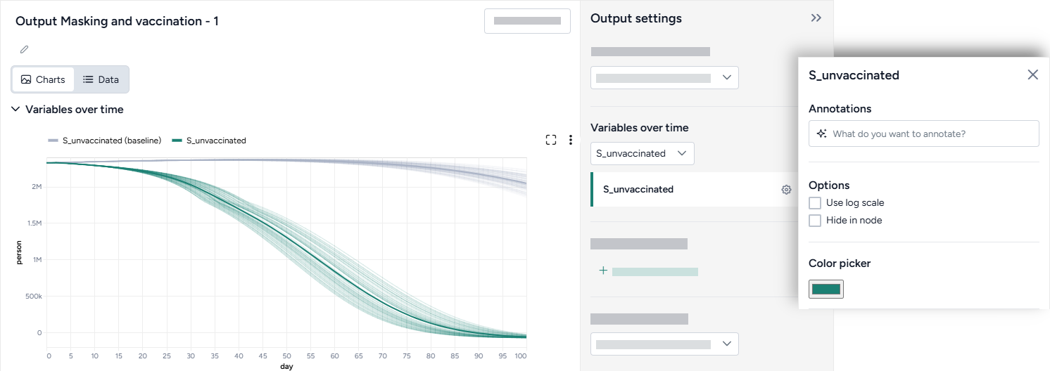
-
Comparison charts
The comparison charts let you plot two or more parameters, model states, or observables to visualize how they differ over the course of the simulation.
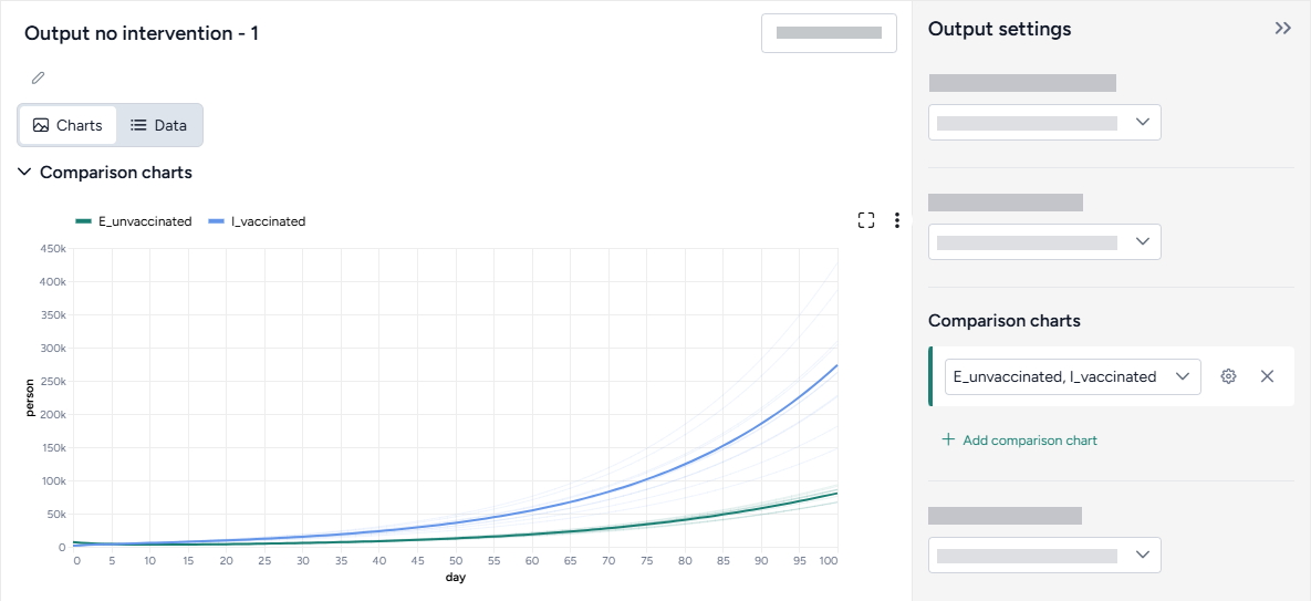
To access the following options for comparison charts, click Options in the Output settings.
Comparison method
Split the selected variables into separate Small multiples charts. You can further customize the small multiples charts to show the Same Y axis for all charts or Show before and after plots of the variables.
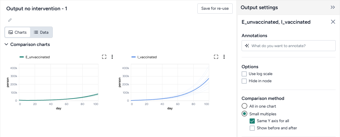
Use multiple charts if the variables you want to compare have very different ranges or values.
Normalization
Normalize data by total strata population to accurately assess the impact on each group regardless of size. With this option selected, the y-axis shows percentages, enabling comparisons across demographic segments by accounting for population size differences.
The equations used to normalize the charts appear below the setting.
-
Sensitivity analysis
Sensitivity analysis charts show how changes in model parameters affect the outcome variables of interest. For more information, see Sensitivity analysis.
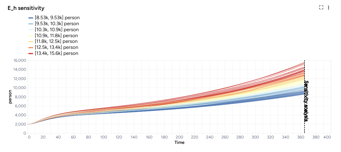
Sensitivity analysis graph showing the number of humans exposed to Mpox at day 365
Access the Output settings
Settings for the various chart types are available in the Output settings panel.
- Click Expand to expand the Output settings.
Choose which variables to plot
- Select the variables from the dropdown list.
Access additional chart settings
Some chart sections let you select additional options for each chart or variable. To access these settings:
- Click Options .
Annotate charts
Adding annotations to charts helps highlight key insights and guide interpretation of data. You can create annotations manually or using AI assistance.
Display options
You can customize the appearance of your charts to enhance readability and organization of the results.
Change the chart scale
By default, charts are shown in linear scale. You can switch to log scale to view large ranges, exponential trends, and improve visibility of small variations.
- Select or clear Use log scale.
Hide in node
The variables you choose to plot appear in the results panel and as thumbnails on the Simulate operator in the workflow. You can hide the thumbnail preview to minimize the space the Simulate node takes up.
- Select Hide in node.
Change parameter colors
You can change the color of any variable on the interventions over time, variables over time, and sensitivity charts to make your charts easier to read.
- Click the color picker and choose a new color from the palette or use the eye dropper to select a color shown on your screen.
Save charts
You can save Simulate charts for use outside of Terarium. Download charts as images that you can share or include in reports, or access structured JSON that you can edit with Vega .
Save a chart for use outside Terarium
- Click and then choose one of the following options:
- Save as SVG
- Save as PNG
- View source (Vega-Lite JSON)
- View compiled Vega (JSON)
- Open in Vega Editor
Data
An interactive table of simulation results enables you to explore model state and parameter values across various samples and timepoints, providing a detailed view of how these values evolve throughout the simulation.
View simulation data
- Click Data.
Troubleshooting
Recommended run settings
It's recommended you run simulations on the Normal Preset using the dopri5 Solver method.
Uncertainty and number of samples
If your models have no uncertainty in parameter values, only one sample is needed. Change Number of samples to 1 (the default is set to 100).
Simulation length and number of samples
If you plan to run your simulation for a long time or with a large number of samples (for example, End time or Number of samples > 100), set them to a lower value (10 or 20) first and run a check for errors.
Error messages
PyCIEMSS error messages should offer guidance on how to proceed. Error messages from Pyro or torchdiffeq may be less clear.
Cholesky factorization
If you see a message referencing Cholesky factorization (including The factorization could not be completed because the input is not positive-definite):
- There is an issue with the model, likely a model state blowing up to infinity or rapidly decreasing to negative infinity. Go back and check your model equations and configuration. Make sure the flow between compartments is correct, and then try adjusting your parameter values or initial conditions (are they too big?).
AssertionError
If the simulation fails and shows an AssertionError: underflow in dt 0.0 error, the configuration has made the model unsolvable with the selected solver Method. This often happens with the dopri5 solver method.
- Workaround: Try using a different solver method, such as rk4 or euler. These solvers are be less efficient than dopri5, but they are also less likely to get caught in an unworkable state
Sensitivity analysis
You can conduct a sensitivity analysis to determine how changes in model parameters affect the outcome variables of interest. For example, you can see how varying vaccination rates and transmission impact hospitalizations.
The sensitivity analysis is performed within the Simulate operator.
Build a sensitivity analysis workflow
You can build a sensitivity analysis workflow manually or use a template to automatically set up the required components.
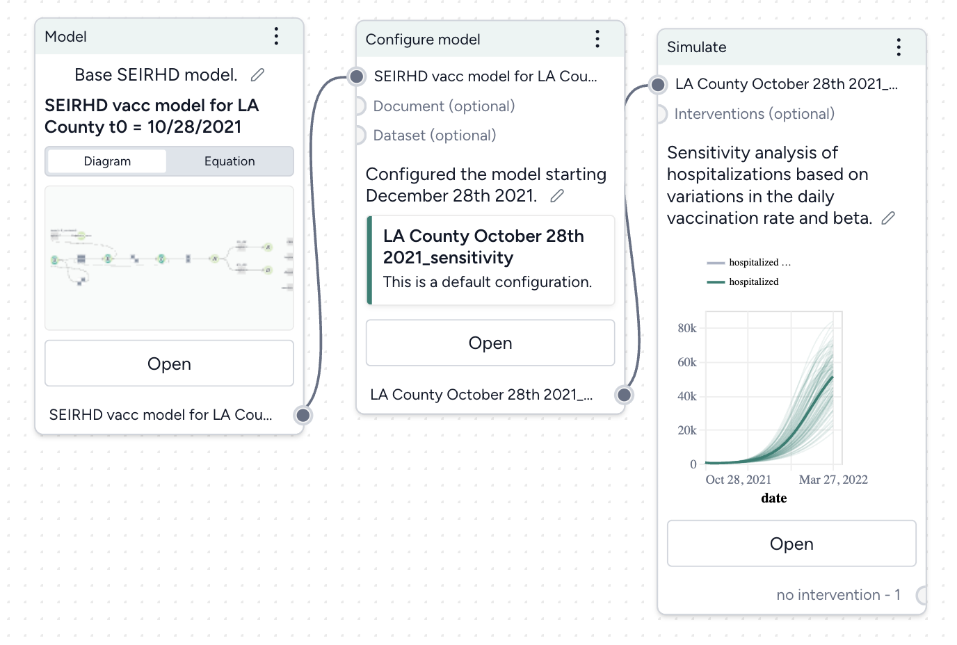
Before you get started, you'll need a:
- Model.
-
Tip
In your model configuration, make sure the parameters you want to analyze have uncertainty in their values.
Once you've set up and run the workflow, you'll have a set of sensitivity analysis simulation results, which you can use as a dataset.
Create a sensitivity analysis workflow from a template
- In the Workflows section of the Resources panel, click New.
- Select Sensitivity analysis.
-
Give the workflow a unique name.
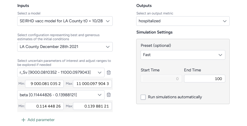
-
Choose the inputs for the analysis:
- Select the model and configuration you want to simulate.
-
Select the model parameters you're interested in. If needed, edit the Min and Max values to define the uncertainty around a parameter.
Note
If you adjust a parameter's uncertainty, Terarium automatically makes a copy of the selected model configuration and applies your edits to the new version.
-
Select the model states you want to visualize.
- Click Create.
Manually create a sensitivity analysis workflow
- Add your model to a workflow, hover over its output, and click Link > Configure model.
- Set the initial values for state variables and parameters. Make sure to apply uncertainty to your parameters of interest.
- Hover over the output of the Configure model operator and click Link > Simulate.
Conduct a sensitivity analysis
Once you've built your workflow, you can edit the Simulate run and output settings to generate the sensitivity analysis.
Conduct a sensitivity analysis
- On the Simulate operator, click Open.
- Select the Simulate run settings.
- Click Run to start the simulation.
Edit the sensitivity analysis output settings
- Click Expand to expand the Output settings.
- In the Sensitivity analysis section, complete the sentence to choose the outcomes and parameters to analyze:
- Outcomes of interest: Choose the model states or observables you're interested in. Selecting more than one outcome of interest creates a unique sensitivity analysis for each selection.
- Choose the timepoint you're interested in:
- Value at timepoint: Enter the timepoint of interest.
- Peak value: The timepoint at which the selected outcome is highest.
- Peak timepoint: The last timepoint.
- Model parameters: Choose the parameters whose impact your want to understand. Each selected parameter is compared against itself and all other selected parameters.
Understand sensitivity analysis results
The results of each analysis are represented as a sensitivity analysis graph, a sensitivity score ranking chart, and a set of parameter comparisons.
In the sensitivity analysis graph, color coding represents variations in the output variable (such as hospitalizations or case counts) across different parameter values or combinations. Cool colors represent lower values of the output variable, while warm colors represent higher values.
The sensitivity score ranking chart shows how much each parameter influences the outcome. The bar chart shows which parameters have the greatest effect, with values ranging from -1 to 1, indicating the direction and magnitude of impact on the outcome.
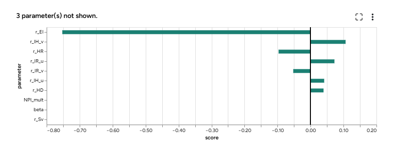
Note
- The sensitivity score chart lists up to the top 20 parameters.
- Parameters with no uncertainty are not included in the sensitivity score ranking.
In the parameter comparisons:
- The x and y-axes represent the parameters being varied (such as vaccination rate and transmission rate). Each point on the graph corresponds to a specific combination of parameter values.
- The color gradient reveals transitions across the graph. Areas with cool colors represent parameter combinations that lead to less severe outcomes, while warm colors highlight conditions where outcomes worsen.
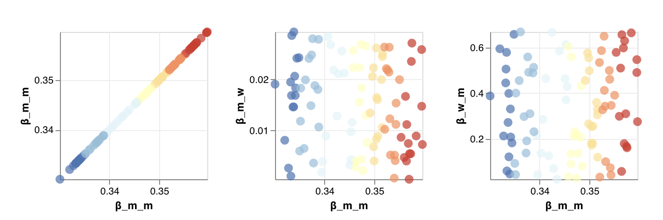
Customize the parameter comparison charts
You can either view the comparisons as scatterplots to examine detailed relationships and outliers in your data or as heatmaps to visualize overall trends and patterns.
- Click Expand to expand the Output settings.
- In the Sensitivity analysis section, select Scatter or Heatmap.
Calibrate a model
Calibration lets you improve the performance of a model by updating the value of configuration parameters. You can calibrate a model with a reference dataset of observations and an optional intervention policy representing historical events that occur during the time period of the reference dataset.
This operation essentially takes prior distribution over the parameters (your knowledge of the world at the first timepoint) and infers posterior distributions over the same, representing the best estimate of the state of the world again but conditioned on data.
Calibrate operator
In a workflow, the Calibrate operator takes a model configuration, a dataset, and optional interventions as inputs. It outputs a calibrated model configuration.
Tip
At least one parameter in the configuration must be defined as a uniform distribution and the dataset must have a column named "Timestamp" with values 0, 1, 2, ... indexing all the timepoints.
Once you've completed the calibration, the thumbnail preview shows the results charts.
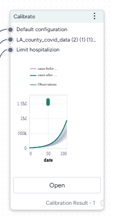
-
Inputs
- Model configuration
- Dataset
- Interventions (optional)
-
Outputs
Calibrated model configuration
Add a Calibrate operator to a workflow
-
Do one of the following actions:
- On an operator that outputs a model configuration, click Link > Calibrate.
- Right-click anywhere on the workflow graph, select Simulation > Calibrate, and then connect a model configuration and a dataset to the Calibrate input.
Calibrate a model
The Calibrate operator allows you to define how to:
Open a Calibrate operator
- Make sure you've connected a model configuration and a dataset to the Calibrate operator.
- Click Open.
Map dataset columns and model variables
To begin, map the observed data (such as number of cases) to the corresponding model states (such as detected cases).
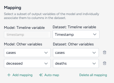
Only relevant variables need to be mapped. For example, if the model includes susceptible and recovered states, but the data only includes infected, you only need to map the infected state. States like susceptible populations that are typically not observed may not be mappable.
Automatically map the dataset and model configuration
If you enriched the model and dataset with concepts, click Auto map to speed the alignment process.
- Click Auto map.
- Review and edit the mappings as needed.
Manually map between the data and model configurations
- Select the Timestamp column from the dataset.
-
For each variable of interest:
- Click Add mapping.
- Select the corresponding state from the model configuration.
Configure the run settings
The Calibrate run settings allow you to fine-tune the time frame, solver behavior, and inference process. By adjusting these settings, you can balance performance and precision.
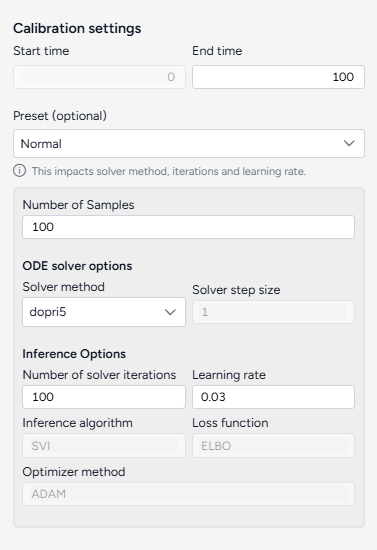
Configure the run settings
The run presets help you quickly choose between fast calibrations, which process quickly but are less accurate, and the normal setting, which is slower but more precise.
- Choose the Start and End time.
- Select a Preset, Fast or Normal.
Advanced settings
Using the following advanced settings, you can further optimize the computational efficiency and thoroughness of the calibration:
- Number of samples: Number of calibration attempts made to explore the parameter space and identify the best fit.
- ODE solver options determine the approach for solving the system's equations during calibration:
- Solver method: dopri5 provides more accurate results with finer calculations, while euler performs simpler, faster calculations.
- Solver step size: Interval between calculation steps, influencing precision and computational cost.
- Inference options control how model parameters are estimated during calibration:
- Number of solver iterations: Number of steps to take to converge on a solution.
- Learning rate: Step size for updating parameters during the optimization process.
- Inference algorithm: Stochastic Variational Inference (SVI), which estimates parameters probabilistically.
- Loss function: Evidence Lower Bound (ELBO), which guides parameter updates by balancing data fit and model complexity.
- Optimize method: ADAM, an algorithm for efficient parameter updates.
Tip
Consider using minimum settings—such as end time 3, number of samples at 1, and the euler solver method—to check whether the calibration can run to completion with the given mapping.
Create the calibrated configuration
Once you've configured all the calibration settings, you can run the operator to generate a new calibrated configuration. The new configuration becomes a temporary output for the Calibrate operator; you can connect it to other operators in the same workflow. If you want to use it in other workflows, you can save it for reuse.
Create a new calibrated configuration
- Click Run.
Choose a different output for the Calibrate operator
- Use the Select an output dropdown.
Understand the results
When the calibration is complete, Terarium creates an AI-generated description of the results.
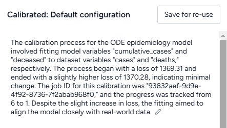
Results are also presented as a series of customizable charts that show:
-
Loss
The loss chart shows the error between the model's output and the calibration data. A decreasing loss indicates successful calibration.
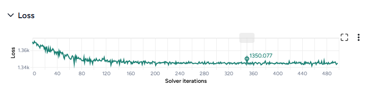
-
Parameter distributions
The parameter distribution plots show the range of parameter values before (grey) and after (green) calibration. A table below the plot also shows the mean and variance.
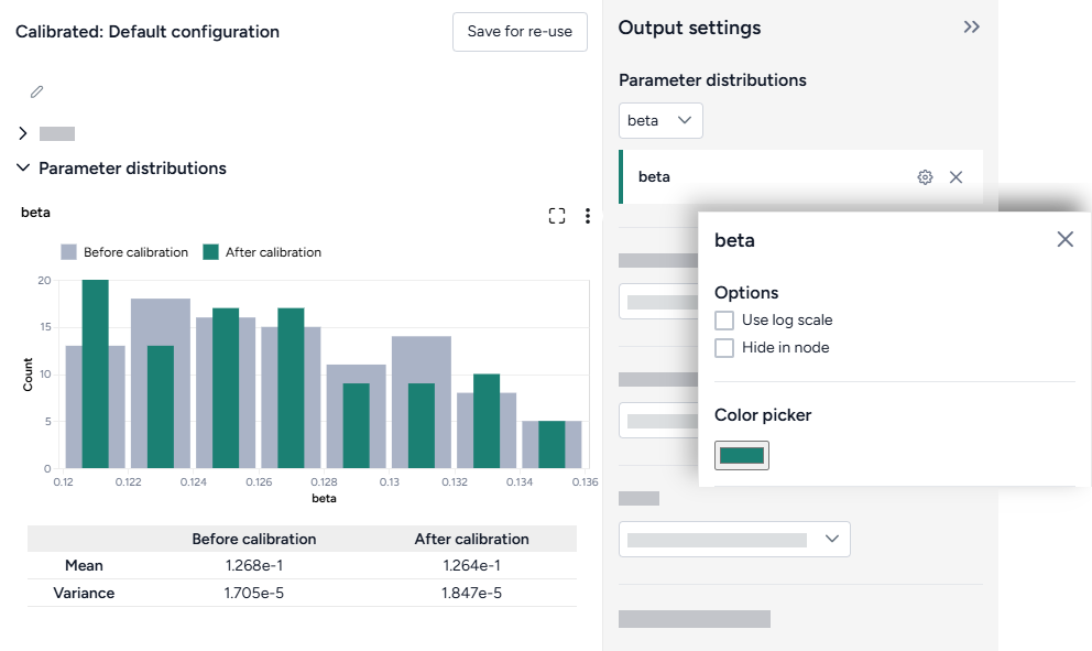
-
Interventions over time
The interventions over time charts show any selected interventions before (grey) and after (green) calibration.
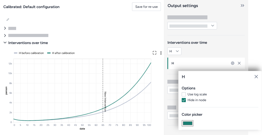
-
Variables over time
To aid visual validation, the variables over time charts compare the effects of calibration for state variables, observables, and the historical data.
- The grey line represents the model before calibration.
- The colored line represents the model after calibration.
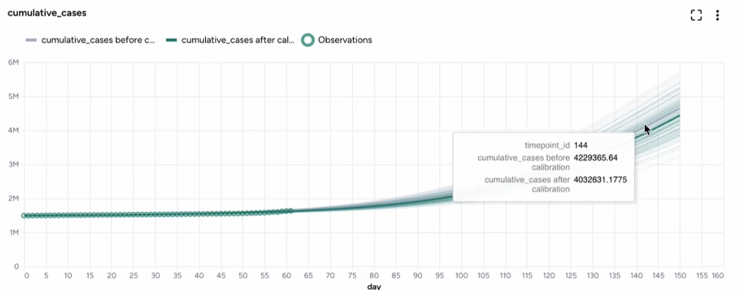
-
Error
The error plots show the mean absolute error (MAE) for each variable of interest.
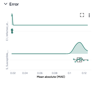
-
Comparison charts
The comparison charts let you plot two or more parameters, model states, or observables to visualize how they changed after calibration.
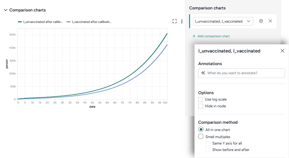
Additional options for comparison charts let you split the selected variables into separate small multiples charts. You can further customize the small multiples charts to show the same Y axis for all charts or incorporate plots of the variables before calibration.
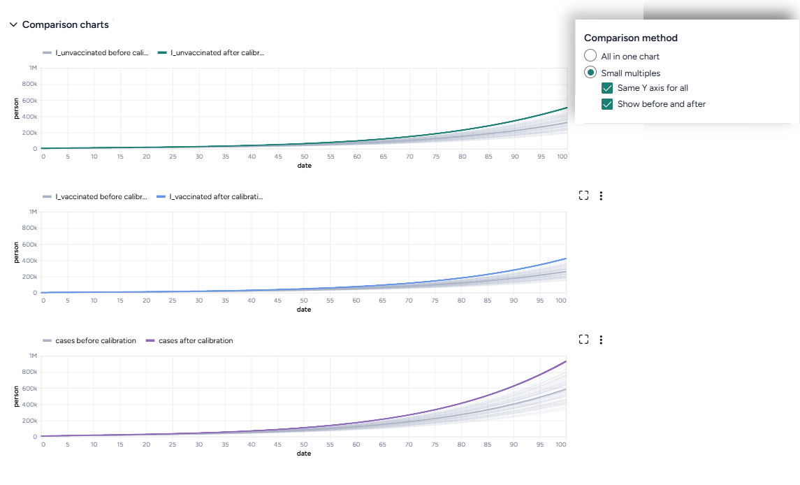
Access the Output settings
Settings for the various chart types are available in the Output settings panel.
- Click Expand to expand the Output settings.
Choose which variables to plot
- Select the variables from the dropdown list.
Access additional chart settings
Some chart sections let you select additional options for each chart or variable. To access these settings:
- Click Options .
Annotate charts
Adding annotations to charts helps highlight key insights and guide interpretation of data. You can create annotations manually or using AI assistance.
Add annotations that call out key values and timesteps
To highlight notable findings, you can manually add annotations that label plotted values at key timesteps on loss, interventions over time, variables over time, and comparison charts.
- Click anywhere on the chart to add a callout.
- To add more callouts without clearing the first one, hold down Shift and click a new area of the chart.
Prompt an AI assistant to add chart annotations
You can prompt an AI assistant to automatically create annotations on the variables over time and comparison charts. Annotations are labelled or unlabelled lines that mark specific timestamps or peak values. Examples of AI-assisted annotations are listed below.
-
Describe the annotations you want to add and press Enter.
Draw a vertical line at day 100Draw a line at the peak S after calibrationDraw a horizontal line at the peak of default configuration Susceptible after calibration. Label it as "important"Draw a vertical line at x is 10. Don't add the labelDraw a line at x = 40 only after calibration
Display options
You can customize the appearance of your charts to enhance readability and organization of the results.
Change the chart scale
By default, charts are shown in linear scale. You can switch to log scale to view large ranges, exponential trends, and improve visibility of small variations.
- Select or clear Use log scale.
Hide in node
The variables you choose to plot appear in the results panel and as thumbnails on the Calibrate operator in the workflow. You can hide the thumbnail preview to minimize the space the Calibrate node takes up.
- Select Hide in node.
Change parameter colors
You can change the color of any variable on the parameter distribution, interventions over time, and variables over time charts to make your charts easier to read.
- Click the color picker and choose a new color from the palette or use the eye dropper to select a color shown on your screen.
Save charts
You can save Calibrate charts for use outside of Terarium. Download charts as images that you can share or include in reports, or access structured JSON that you can edit with Vega .
Save a chart for use outside Terarium
- Click and then choose one of the following options:
- Save as SVG
- Save as PNG
- View source (Vega-Lite JSON)
- View compiled Vega (JSON)
- Open in Vega Editor
Troubleshooting
Recommended run settings
It's recommended you run calibrations using the dopri5 Solver method.
Simulate first
Before you calibrate, confirm that your model can be simulated.
Uncertainty and number of samples
If your model has uncertainty in parameter values, only one sample is needed. Change Number of samples to 1 (the default is set to 100).
Simulation length and number of samples
If you plan to simulate your calibrated model for a long time or with a large number of samples (for example, End time or Number of samples > 100), set them to a lower value (10 or 20) first and run a check for errors.
Error messages
PyCIEMSS error messages should offer guidance on how to proceed. Error messages from Pyro or torchdiffeq may be less clear.
If you see a messages referencing Cholesky factorization (including The factorization could not be completed because the input is not positive-definite) or AssertionError with underflow in dt 0.0:
- If you were able to simulate the model, check that your model and the dataset are on the same scale. Errors are likely if:
- The model assumes a population of 10 million, while the dataset has a population of 1,000.
- The model is normalized to a population of one while the dataset is not.
- Make sure your initial conditions are consistent with your dataset. They don't need to be an exact match, but errors are likely if they are too far off.
Simulate ensemble
More info coming soon.
Simulate ensemble operator
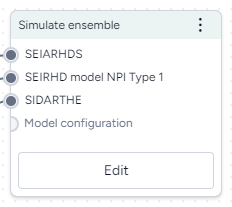
-
Inputs
Model configurations
-
Outputs
Simulation data
Run an ensemble simulation
Run an ensemble simulation
- Configure two or more models.
- Right-click anywhere on the workflow graph and select Simulation > Simulate ensemble.
- Connect the Configure model outputs to the Simulate ensemble inputs.
- Click Open.
- Create a mapping between the state variables of the model configurations.
- Enter custom weights for the model configurations to specify your confidence in them.
- Select a Preset, Fast or Normal.
- Set the time span:
- End time
- Number of timepoints
- Number of samples
- Choose a Solver method, dopri5, rk4, or euler.
- Click Run.
Troubleshooting
Recommended run settings
It's recommended you run simulations on the Normal Preset using the dopri5 Solver method.
Simulate each model first
Try simulating each model independently to confirm the models are composed and configured correctly.
Relative certainty
Set the Relative certainty in the Model weights to 1 for each model. When using this setting, proceed slowly and cautiously. To include a preference for one model over the others, start by increasing its Relative certainty to 2, then 3, and so on.
Uncertainty and number of samples
If your models have no uncertainty in parameter values, only one sample is needed. Change Number of samples to 1 (the default zis set to 100).
Simulation length and number of samples
If you plan to run your simulation for a long time or with a large number of samples (for example, End time or Number of samples > 100), set them to a lower value (10 or 20) first and run a check for errors.
Error messages
PyCIEMSS error messages should offer guidance on how to proceed. Error messages from Pyro or torchdiffeq may be less clear.
Cholesky factorization
If you see a message referencing Cholesky factorization (including The factorization could not be completed because the input is not positive-definite):
- If you successfully simulated each model independently, check that the models are on the same scale and have similar initial conditions. Errors are likely if:
- One model assumes a population of 10 million, while another has a population of 1,000.
- One model is normalized to a population of one while the others are not.
AssertionError
If the simulation fails and shows an AssertionError: underflow in dt 0.0 error, the configuration has made the model unsolvable with the selected solver Method. This often happens with the dopri5 solver method.
- Workaround: Try using a different solver method, such as rk4 or euler. These solvers are be less efficient than dopri5, but they are also less likely to get caught in an unworkable state
Calibrate ensemble
You can jointly calibrate multiple models as an ensemble. In an ensemble calibration:
- Each member model is independently calibrated against the same time-series dataset representing historical observations.
- The models are recalibrated as a single ensemble, with loss or prediction error calculated as a linearly weighted sum of the different model outputs and dataset features.
The result is a joint set of calibrated model configurations that may generate predictions with lower error than than individual models or their independently calibrated configurations.
Ensemble calibration essentially allows a search for configuration solutions where the member models can specialize to different features or time periods of the given dataset. This is analogous to a high-performing random forest regressor which can be constructed from multiple weak-learning decision trees.
Calibrate ensemble is powered by the ensemble_calibrate function of the PyCIEMSS package. An example of how it can be used programmatically can be found in this Jupyter notebook.
Tip
You can quickly create an ensemble calibration using the Calibrate an ensemble model workflow template.
Calibrate ensemble operator
In a workflow, the Calibrate ensemble operator takes two or more model configurations and a dataset as inputs. It outputs a calibrated dataset.
Once you've completed the calibration, the thumbnail preview shows the calibrated ensemble variables over time.
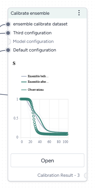
-
Inputs
- Two or more model configurations
- Dataset (with timepoints)
-
Outputs
Calibrated dataset
Add a Calibrate ensemble operator to a workflow
-
Do one of the following actions:
- On an operator that outputs a model configuration, click Link > Calibrate ensemble.
- Right-click anywhere on the workflow graph, select Simulation > Calibrate ensemble, and then connect two or more model configurations and a dataset to the Calibrate ensemble input.
Calibrate ensemble
The Calibrate ensemble operator allows you to define how to:
- Map your model configurations and dataset.
- Assign your level of confidence in each model.
- Choose how to run the calibration.
Open a Calibrate ensemble operator
- Make sure you've connected two or more model configurations and a dataset to the Calibrate ensemble operator.
- Click Open.
Map dataset columns and model variables
To begin, create a mapping between the calibration data and the model configurations by selecting features and corresponding outcomes that are represented by each model.
Example
Map dataset columns current number of hospitalized cases and cumulative number of deaths to threatened (T) and extinct (E) populations in a SIDARTHE model or hospitalizations (H) and deaths (D) in a SEIQHRD-type model
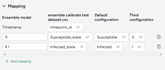
It's not necessary to map between every dataset feature to a set of model outcomes. For example, susceptible or exposed populations in SEIR-type models do not correspond to readily observed or reported values.
Tip
High-quality case, death, and hospitalization data for COVID-19 is available on the COVID-19 Forecast Hub GitHub repository. If a model selected for ensemble calibration does not have a state variable that corresponds well to these observations, add an observable using Edit model notebook.
Tip
State variables in compartmental models usually represent prevalence of disease conditions. Literature and data repositories often provide only daily incident or cumulative estimates. Use the Transform dataset operator to convert from incidence to prevalence values.
You can also use the Edit model operator to add new "controlled production" transitions and create new state variables that are cumulative equivalents.
For example, define a cumulative equivalent (Icum) of the number of infected individuals (I) for a SIR-type model by adding a controlled production where the:
- Outcome is
Icum. - Controller is
I. - Rate law is
I.
The resulting equation in this case should be d Icum(t) / dt = I(t) or Icum(t) = int I(t) dt.
Create a mapping between the calibration data and the model configurations
- Select the Timestamp column from the dataset.
-
For each variable of interest:
- Click Add mapping.
- Enter a unique name for the variable in the ensemble model.
- Select the corresponding state from each of the model configurations.
Assign model weights
Model weights are the parameters used to linearly sum the model outcomes in the ensemble. They represent how much each model contributes to the ensemble.
Because Calibrate ensemble is Bayesian inference process, the model weights are not single values but are represented by a Dirichlet distribution of order K, where K is the number of models in the ensemble. This distribution has parameters a_1, a_2, ..., a_K that control where and how much mass is concentrated at different possible combinations of normalized model weights (w_1, w_2, ..., w_k).
In the interface, the Dirichlet alpha parameters a_k are exposed as Relative uncertainty. Selecting from 0 to 10 allows you to express your confidence in each of the models and find an ensemble solution that potentially produces better predictions.
Assign model weights
- For each model, select a value from
1(low) to10(high) using the Relative certainty dropdown.
- If you don't know which models are better and should have more weight, assign equal medium weights (
5). This is equivalent to initially assuming a flat Dirichlet distribution where all model weight combinations are equally probable. This is the default and recommended option. - Assign a high weight (
10) to one or more models that you believe produce the best predictions. Calibrate ensemble searches for solutions that prioritize the contribution of these models. - Assign a low weight (
1) to models that you believe are less reliable. Their contributions are reduced in the ensemble calculation.
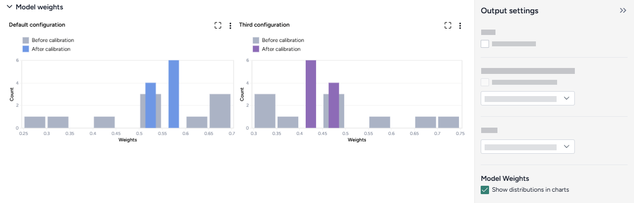
Configure the run settings
The Other settings control the time period of interest and behavior of the underlying ODE solver and optimizer. You can select a preset (Fast or Normal) or adjust these settings individually to balance between run time and precision.
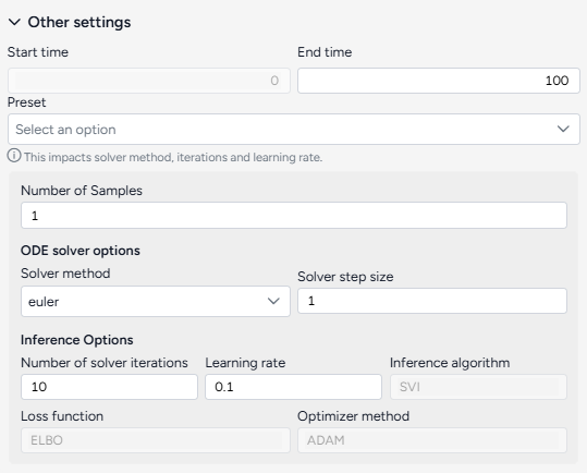
Quickly configure the run settings
- Choose the Start time and End time to specify the timepoints to be simulated.
- Select a Preset, Fast or Normal.
Advanced settings
Using the following advanced settings to control how fast or precise the calibration should be:
- Number of samples: Number of point estimates to be made on the posterior distribution (model parameters and weights) for the pre and post-calibration simulations.
- ODE solver options determine the approach for solving the equations of the model during calibration:
- Solver method: dopri5 returns the best results while euler is faster but less accurate (more details).
- Solver step size: Size of the time interval used to integrate the solution. Larger values are faster but less accurate (only needed by the euler method).
- Inference options control the behavior of the inference algorithm that minimizes the calibration error:
- Number of solver iterations: The number of calibration steps.
- Learning rate: Step size for updating parameter values during calibration.
- Inference algorithm: Stochastic Variational Inference (SVI), which estimates the parameters probabilistically.
- Loss function: Evidence Lower Bound (ELBO), which guides parameter updates by balancing data fit and model complexity.
- Optimizer method: algorithm for updating parameter values, ADAM by default.
Tip
Consider using minimum settings - such as the end time at 3, the number of samples at 1, and the solver method at euler - to check whether the calibration can run to completion with the given mapping.
Create and save the calibrated dataset
Once you've configured the settings, you can run the operator to generate a new calibrated dataset. The new dataset becomes a temporary output for the Calibrate ensemble operator. You can connect it to other operators in the same workflow.
Create a new calibrated dataset
- Click Run.
Choose a different output for the Calibrate ensemble operator
- Use the Select an output dropdown.
Understand the results
Ensemble calibration results are presented as a series of charts that show:
Access the Output settings
Additional settings for the various chart types are available in the Output settings panel.
- Click Expand to expand the Output settings.
Save a chart for use outside Terarium
You can save Calibrate ensemble charts for use outside of Terarium. Download charts as images that you can share or include in reports, or access structured JSON that you can edit with Vega .
- Click and then choose one of the following options:
- Save as SVG
- Save as PNG
- View source (Vega-Lite JSON)
- View compiled Vega (JSON)
- Open in Vega Editor
Add annotations that call out key values and timesteps
To highlight notable findings, you can manually add annotations that label plotted values at key timesteps on loss and ensemble variable charts.
- Click anywhere on the chart to add a callout.
- To add more callouts without clearing the first one, hold down Shift and click a new area of the chart.
Note
Ensemble variable charts also support AI-generated annotations.
Loss
The loss chart shows the error between the ensemble model outputs and the calibration data. A monotonic and exponential decrease in loss values indicates convergence and a successful calibration.
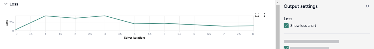
Show or hide the loss chart
- Select or clear Show loss chart.
Tip
If the loss doesn't decrease to a plateau, the calibration algorithm may be struggling to converge on a solution. Failure to converge could indicate that the model outputs are not good matches to the calibration data. Consider reducing the complexity of the problem by:
- Adjusting the values of the input model configurations to approximate a solution.
- Removing the larger or least trustworthy model configurations.
Ensemble variables over time
To aid visual validation, the Ensemble variables over time charts compare the effects of calibration for each state variable and the historical data.
- The grey line represents the model before calibration.
- The colored line represents the model after calibration.
- Circles represent observations from the historical data.
The Output settings panel has several options that let you customize the scale and display of the charts. You can also use an AI assistant to generate chart annotations that highlight key data points.
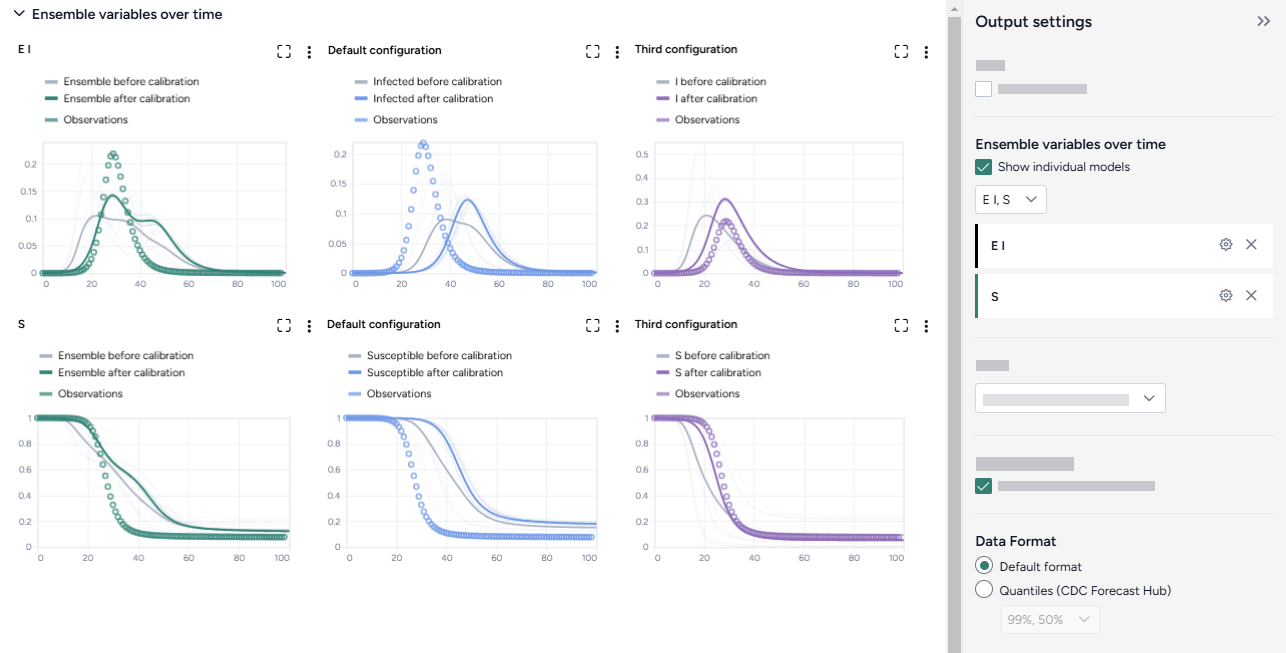
Choose which model states to plot
- Select the model states from the dropdown list.
Show charts for each model configuration
You can view individual charts for all the models that contribute to the ensemble model as small multiples.
- Click Show individual models.
Change the data format
The data format controls how the ensemble variable charts are drawn.
- Choose the Data format:
- Default: Include the historical observations in the plot.
- Quantiles (CDC Forecast Hub): Omit the historical observations and draw filled shapes to represent quantiles ranging from 50$ndash;90%.
Additional chart settings are available for each of the state variables.
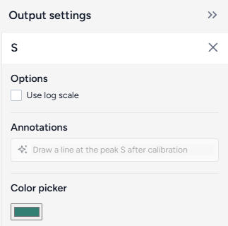
Access additional chart settings
- Click Options .
Change the chart scale
By default, ensemble variable charts are shown in linear scale. You can switch to log scale to view large ranges, exponential trends, and improve visibility of small variations.
- Select or clear Use log scale.
Change variable colors
You can change the color of any model state to make your charts easier to read.
- Click the color picker and choose a new color from the palette or use the eye dropper to select a color shown on your screen.
Prompt an AI assistant to add chart annotations
You can prompt an AI assistant to automatically create annotations on the ensemble variable charts. Annotations are labelled or unlabelled lines that mark specific timestamps or peak values. Examples of AI-assisted annotations are listed below.
-
Describe the annotations you want to add and press Enter.
Draw a vertical line at day 100Draw a line at the peak S after calibrationDraw a horizontal line at the peak of default configuration Susceptible after calibration. Label it as "important"Draw a vertical line at x is 10. Don't add the labelDraw a line at x = 40 only for ensemble after calibration
Error
The error plots show the mean absolute error (MAE) for each model and variable of interest.
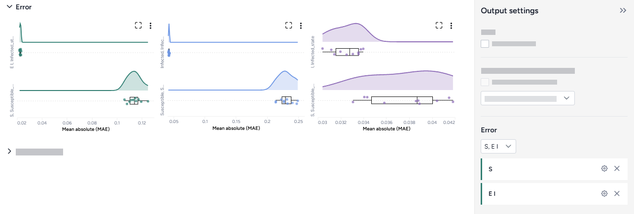
Change the chart scale
By default, error charts are shown in linear scale. You can switch to log scale to view large ranges, exponential trends, and improve visibility of small variations.
- Click Options .
- Select or clear Use log scale.
Model weights
The model weights charts display one-dimensional projections of the Dirichlet distribution of the weights for each model, before and after the calibration.
Generally, a good calibration takes a broad distribution (a low-certainty prior) and returns a narrow distribution (a high-certainty posterior, conditioned on the calibration data).
To show or hide the model weights charts
- Select or clear Show distributions in charts.
Troubleshooting
Recommended run settings
It's recommended you run calibrations using the dopri5 Solver method.
Calibrate each model first
Try calibrating each model to your dataset independently.
Relative certainty
Set the Relative certainty in the Model weights to 1 for each model. When using this setting, proceed slowly and cautiously. To include a preference for one model over the others, start by increasing its Relative certainty to 2, then 3, and so on.
Uncertainty and number of samples
If your models have no uncertainty in parameter values, only one sample is needed. Change Number of samples to 1 (the default is set to 100).
Simulation length and number of samples
If you plan to simulate your calibrated ensemble model for a long time or with a large number of samples (for example, End time or Number of samples > 100), set them to a lower value (10 or 20) first and run a check for errors.
Error messages
PyCIEMSS error messages should offer guidance on how to proceed. Error messages from Pyro or torchdiffeq may be less clear.
If you see a messages referencing Cholesky factorization (including The factorization could not be completed because the input is not positive-definite) or AssertionError with underflow in dt 0.0:
- If you successfully calibrated each model independently, check that the models and the dataset are on the same scale. Errors are likely if:
- One model assumes a population of 10 million, while another (or the dataset) has a population of 1,000.
- One model (or the dataset) is normalized to a population of one while the others are not.
- Make sure your initial conditions are similar to each other and consistent with your dataset. They don't need to be an exact match, but errors are likely if they are too far off.
Ended: Simulation
Annotate your work
You can capture and save insights you've gained during your modeling processes:
- Directly on the operator where you discovered them.
- On the workflow canvas.
- In the project overview.
- On charts generated through simulations and calibrations.
Add a note to a workflow operator
You can add notes to any operator in the workflow graph.
Add a note to a workflow operator
- Perform one of the following actions:
- On the operator in the workflow graph, click > Add a note
- In the operator details, click Add a note.
- Add your note and press Enter.
Create a project overview
The project overview page is another space for you to capture notes and summarize the findings and processes used in your modeling workflows.
For example, to assist with publishing a paper, you could organize insights into sections such as Abstract, Intro, Methods, Results, Discussion, or References.
Saving your overview
Terarium automatically saves the state of your overview as you make changes.
Edit the project overview
- In the Resources panel, click Overview.
- Enter your insights in the text field. Use the style bar to format your text.
Add an annotation to the workflow canvas
You can add notes directly to the canvas to provide more context for the modeling decisions you've made in your workflow.
Add an annotation to the workflow canvas
- Right-click on the workflow canvas and select Text block.
- Double-click
annotation text, enter some text, and press Ok. - Click and drag the annotation to a new location if needed.
Annotate charts
Adding annotations to charts helps highlight key insights and guide interpretation of data. You can create annotations manually or using AI assistance.
Add annotations that call out key values and timesteps
To highlight notable findings, you can manually add annotations that label plotted values at key timesteps.
- Click anywhere on the chart to add a callout.
- To add more callouts without clearing the first one, hold down Shift and click a new area of the chart.
Prompt an AI assistant to add chart annotations
You can prompt an AI assistant to automatically create annotations on the variables over time and comparison charts. Annotations are labelled or unlabelled lines that mark specific timestamps or peak values. Examples of AI-assisted annotations are listed below.
- In the Output settings, click Options .
-
Describe the annotations you want to add and press Enter.
Draw a vertical line at day 100Draw a line at the peak S after calibrationDraw a horizontal line at the peak of default configuration Susceptible after calibration. Label it as "important"```{ .text .wrap } Draw a line at x = 40 only for ensemble after calibrationDraw a vertical line at x is 10. Don't add the label
Integrated subsystems ↵
Integrated subsystems
More info coming soon.
TDS
More info coming soon.
AMR
More info coming soon.
Knowledge extraction
More info coming soon.
Create model from code
-
Documentation
-
Source code
Create model from equations
Model Service provides REST-API wrappers for creating, manipulating, and transforming ODE/Petrinet models.
-
Documentation
-
Source code
Transform dataset
-
Documentation
-
Source code
Modeling
More info coming soon.
Edit model
-
Documentation
-
Source code
Validate configuration
-
Documentation
-
Source code
Stratify model
-
Documentation
-
Source code
Compare models
-
Documentation
-
Source code
Simulation
More info coming soon.
Simulate
-
Documentation
-
Source code
Calibrate
-
Documentation
-
Source code
Optimize
-
Documentation
-
Source code
Simulate ensemble
-
Documentation
-
Source code
Calibrate ensemble
-
Documentation
-
Source code
Beaker
Beaker is a custom Jupyter kernel that can integrate notebooks into any web application, either as custom-designed notebooks or through native UI elements that run code in any language. The Beaker AI agent is powered by a large language model (LLM) that can generate code to populate notebooks or run code in the background.
The Beaker kernel connects to the Terarium Data Service to enable users to get contextual answers to natural language questions, automatically generate executable code, and perform scientific modelling processes such visualizing or modifying datasets.
-
Provider
Beaker was developed by Jataware .
-
Documentation
-
APIs
-
Source code
Ended: Integrated subsystems
Glossary ↵
Glossary
A–M
Alignment-
A mapping from the features of a dataset to the state variables, parameters, and initial conditions of a model. The alignment supports constructing configurations of a simulation. The SIR compartmental model and a training dataset with features
truth-incident_cases,truth-incident_deaths,truth-incident_hospitalizationcan have the following model-data alignment:{ "S": null, "I": null, "R": null, "I_obs": null, "N": null, "R_frac": null, "ℜ₀": null, "inc_I_obs": "truth-incident_cases", "inc_D": "truth-incident_deaths", "inc_H": "truth-incident_hospitalization" }Note
Incident refers to new occurrences, while "prevalent" refers to current (new and preexisting) occurrences.
Calibration-
A form of statistical inference for determining or updating the value (point estimate or posterior distribution) of model parameters given a reference dataset of observations. The result is typically selected to balance trade-offs between consistency with the modeler's expert knowledge and the "fit" of model observables to the dataset. In advanced cases, other selection criteria can include robustness to model misspecification, interpretability, focus on one statistical quantity of interest, and data privacy and security.
Configuration-
Any set of values used as input for a simulator. A configuration is a simulation and model-specific representation of a scenario.
Downscaling-
In climate science, the process of combining high-resolution observational data with low-resolution models to generate high-resolution simulation results that would otherwise be too coarse to accurately capture the dynamics of large-scale phenomena such as hurricanes.
Fitting-
See Calibration.
Gene regulatory network
See RegNet.
GNR
See RegNet.
Hyperparameter-
A quantity that's an input of a simulator. Hyperparameters can't be inferred from data and can impact the precision and accuracy of the resulting simulation.
loss,penalty, andtolare hyperparameters of the stochastic gradient descent algorithm . Inference-
See Calibration.
Initial condition-
A parameter that corresponds to the value of a state variable at a starting time point. In a model, there are as many initial conditions as state variables.
S₀,I₀, andR₀are initial conditions of the SIR compartmental model. Lineage graph-
A subgraph of the provenance graph. A lineage graph tracks the versioning of an artifact, containing all the data processing steps that lead to its creation.
Model-
An abstract representation that approximates the behavior of a system. For example, a set of ordinary differential equations can approximate the course of an epidemic.
Model template-
A template is a piece of a model that depicts a common transition for a variable or group of variables. Model templates can be used to quickly edit or create a model. For each model framework, the available model templates make up a list of all the possible states and transitions.
Depending on the modeling framework, available model templates may include:
- Natural conversion
- Natural production
- Natural degradation
- Controlled conversion
- Controlled production
- Controlled degradation
- Grouped controlled conversion
- Grouped controlled production
- Grouped controlled degradation
- Natural replication
- Controlled replication
Modeling-
The process of building a model or a simulation.
Modeling framework-
Examples include PetriNets, gene regulatory networks (regnets), stock and flow diagrams, and agent-based models (ABMs). Terarium uses the JSON serialization schemas defined in the ASKEM Model Representations repository.
N–Z
Observable-
A quantity of a system (and corresponding model) that's measurable as an "observation" data point. The SIR compartmental model has the following observables:
I_obs(observed infected population)N(total population)R_frac(recovered population fraction)ℜ₀(basic reproduction ratio )inc_I_obs(observed incident infection rate)
Observation function-
A function that maps state variables to an observable, capturing knowledge such as the physics of the observation or measurement process and expert heuristics. For example:
I_obs = 0.50 * I
N = S + I + R
R_frac = R / N
ℜ₀ = β * S / γ
inc_I_ob = diff(I_obs(t), t)) * Heaviside(diff(I_obs(t), t))
For convenience, an observation function may refer to observables in many cases.
Operator-
An operator in the workflow graph is a node that can represent a model, dataset, or document or a scientific modeling process that modifies or executes project resources.
Operators that perform scientific modeling processes have two configuration methods. A wizard view exposes the most common configuration options, while a notebook view provides a direct interface to writing and editing executable code. Additionally, an integrated AI assistant can generate code based on natural language input.
Optimization-
The process of determining the values of variables that minimize or maximize some objectives subject to constraints. These variables typically represent possible
interventionsto achieve an outcome (for example, adjusting the duration of a masking policy to reduce the number of hospitalized individuals). In risk-based optimization under uncertainty (RBOUU), the objectives and constraints can be functions of distributions of model parameters and outputs. For example, the constraint that the probability of a super-spreader event never exceeds a threshold value.Note
Fittingcan involve optimization ("optimal fitting" and "constrained optimal fitting") but not necessarily (approximation with a "particle filter"). Parameter-
A fixed quantity of a model. Parameters consist of the constants internal to the model. They can be inferred from data made from observations of the underlying system.
βandγare parameters of the SIR compartmental model and weights of an artificial neural network model. PetriNet-
A PetriNet---or place/transition network---is a modeling framework that represents the dynamic behavior of a system. Circular nodes represent variables or places taken at states or compartments. Square nodes represent transitions. Edges between nodes show the flow of variables or places through various transitions.
A PetriNet could, for example, represent populations of people transitioning between the different states in an SIR (susceptible/infected/recovered) model.
Provenance graph-
A directed graph constructed from all the artifacts created by the workflow (as nodes) and the relations between them (as links):
Relation Type Source Node Type Target Node Type 0 COPIED_FROM Model Model 1 COPIED_FROM ModelRevision ModelRevision 2 GLUED_FROM Model Model ... ... ... 32 IS_CONCEPT_OF Concept Dataset RegNet-
A RegNet---or gene regulatory network (GNR)---is a modeling framework commonly used in systems biology. Nodes (or vertices) represent genes, proteins, or chemicals, while edges represent regulatory relationships or interactions between them.
Result-
The output of a simulation (partial or complete).
Run-
An execution of a simulation.
Scenario-
A natural-language description of the context, problems, or questions that require a modeling and simulation process.
Given a scenario, you can construct a simulation and a configuration through modeling to execute a run and generate a result. During a run, the simulator has states and values (running time, memory usage) incidental to the simulation that are not considered part of the result, but that may influence future model and simulation selection.
Simulating-
The process of executing a simulation on a simulator.
Simulation-
An executed instance of a model. A simulation suggests the behavior of the underlying system under specific conditions. What makes a model executable depends on the details of the model, the simulator, and the goals of the people involved.
Simulator-
A program that runs a model with specific input values and generates output values.
State variable-
A varying quantity of a system and corresponding model. In combination with others, these variables can fully determine the "state" of the underlying system.
S,I, andRare state variables of the SIR compartmental model. Stock and flow-
Stock and flow is a modeling framework commonly used in system dynamics. Nodes represent stocks or reservoirs that accumulate over time. Edges between stocks flow into valves that represent how accumulations change.
Strata model-
A model that captures the fine-grained interactions between the different strata state variables. Examples include infectious contact between subpopulations of different age groups and travel by individuals between different locations.
Stratification-
The process of dividing the populations of a model into subsets (subpopulations or strata), often along demographic characteristics such as age and location. The goal is to include more fine-grained interactions—those between the strata—into the model.
It is herein implemented as a kind of "typed" Cartesian product between the graph representation of a model
Pand that of one or many "strata models"Q. The stratified modelGhas:- A node for every pair of nodes in
PandQof the same type. - A link for every link in
PorQwith the same pair of node types.
- A node for every pair of nodes in
Training-
See Calibration.
Workflow graph-
A data-flow diagram made up of high-level operators that represent resources and scientific modeling processes such as configure model, calibrate model, and simulate model.